
Numerical differentiation
import numpy as np
import matplotlib.pyplot as plt
First derivatives
We seek for approximating $f'$ in $x \in [a,b]\subset \mathbb{R}$ that depends only on values of $f$ in a finite number of points close to $x$.
The two main reasons to do this are:
- We only know the value of $f$ in some points $x$.
- It is cheaper to compute the approximation than the exact value.
The derivative of a function $f$ in $x$ can be defined
$$ f'(x)=\lim_{h\to0}\frac{f(x+h)-f(x)}{h} $$The following approximations
Forward
$$ f'(x)\approx\frac{f(x+h)-f(x)}{h}$$Backward
$$ f'(x)\approx\frac{f(x)-f(x -h)}{h}$$Centered
$$ f'(x)\approx \frac{f(x+h)-f(x-h)}{2h}$$For all the above schemes, the edge problem arises, due to the fact that the finite differences cannot be computed at one or both of the interval borders. For instance, if the forward formula is used we cannot compute the forward approximation because we need $f(b+h)$ that, in general, it is unknown.
Given the function $f(x)=\ln(x)$ in $[1,2]$ and for h = 0.1 and h = 0.01.
- Calculate and plot its exact derivative.
- Compute the approximate derivative, using the forward
df_f, backwarddf_band centereddf_capproximations in equispaced points, with a space between them ofh, in the interval $[1,2]$. You cannot use points outside this interval. Plot it with the exact derivative. - In a new figure, compute and plot the error for every point for the approximations, $\left|f'(x_i)-df_a(x_i)\right|$, where $x_i$ are the points and $a=p,~r$ or $c$.
- Compute and print the global relative error for each approximation using the formula
Hints
- The equispaced points can be obtained, for instance
- Using a loop.
- Using
np.arange. - Using
np.linspace.
- The numerical results can vary slightly depending on the used method.
- The command
np.diff(v)that computes $(v_2-v_1,v_3-v_2,\ldots,v_n-v_{n-1})$ could be useful. - To compute the $2$ norm (euclidean) of a vector
vyou can use the commandnorm. For instance,$$ \mathrm{norm}(v)=\left\Vert v\right\Vert_2= \sqrt{\sum_{i=1}^n v_i^2}$$from numpy.linalg import norm vn = norm(v)
%run Exercise1


We see that the centered scheme gives better results. That is because forward and backward formulas are order 1 formulas and the centered formula is an order 2 formula.
Is it possible to get order 2 approximations for $f'a)$ and $f'(b)$? Yes, if we use a Lagrange interpolation polinomial of $f$ of second degree in $x_0$, $x_1$, $x_2$, with $h\gt 0$ and $x_1 = x_0+h$, $x2 = x_1+h$ and $y_j=f(x_j)$.
Then we have the second order formulas
$$ \begin{array}{l} \mathbf{Forward}\\ f'(x_{0})\approx\dfrac{-3y_{0}+4y_{1}-y_{2}}{2h}\\ \mathbf{Centered}\\ f'(x_{1})\approx\dfrac{-y_{0}+y_{2}}{2h}\\ \mathbf{Backward}\\ f'(x_{2})\approx\dfrac{y_{0}-4y_{1}+3y_{2}}{2h} \end{array} $$They can also be written:
$$ \begin{array}{l} \mathbf{Forward}\\ f'(x)\approx \dfrac{1}{2h}(-3f(x)+4f(x+h)-f(x+2h))\\ \mathbf{Centered}\\ f'(x)\approx \dfrac{1}{2h}(f(x+h)-f(x-h))\\ \mathbf{Backward}\\ f'(x)\approx \dfrac{1}{2h}(f(x-2h)-4f(x-h)+3f(x)) \end{array} $$Given the function $f(x)= x^3 + x ^2 + x$ in $[0,1]$, and h = 0.02
- Compute the approximate derivative of
fusing the centered formula for the inner points and the progressive and regressive order 1 formulas (two points) for $f'(0)$ and $f'(1)$ respectively. - Compute the approximate derivative of
fusing the centered formula for the inner points and the progressive and regressive order 2 formulas (three points) for $f'(0)$ and $f'(1)$ respectively. - Compute and print the global relative error for each approximation in $[0,1]$
- Plot the exact derivative and its approximation.
Hint
To concatenate vectors, you can
- Initialize a vector and fill it with a loop.
- Initialize a vector and fill it with slicing.
v = np.zeros(5)
v[0] = 3.
v[1:4] = np.array([5.,4,3])
v[-1] = 2.
- Use the command
np.concatenate
%run Exercise2.py


Second derivatives
From the interpolating polynomial
$$ p(x)=[y_1]+[y_1,y_2](x-x_1)+[y_1,y_2,y_3](x-x_1)(x-x_2) $$we obtain
$$p''(x_2)=2[y_1,y_2,y_3]= \frac{1}{h^2}(y_1-2y_2+y_3)$$It can also be written:
$$ \begin{array}{l} \mathbf{Centered}\\ f''(x)\approx \dfrac{1}{h^2}(f(x+h)-2f(x)+f(x-h))\quad (1) \end{array} $$Given the function $f(x)=\cos(2\pi x)$ in $[-1,0]$ and h = 0.001
Compute and plot the exact second derivative in $[-1,0]$ and the approximate second derivative using the latter formula. Calculate the relative error of the approximation in the interval $[-1+h,-h]$.
%run Exercise3.py

For $\Omega =[a,b]\times[c,d]\subset \mathbb{R}^2$, consider uniform partitions
\begin{eqnarray*} a=x_1 \lt x_2 \lt \ldots \lt x_{M-1} \lt x_M=b \\ c=y_1 \lt y_2 \lt \ldots \lt y_{N-1} \lt y_N=d \end{eqnarray*}Denote a point by $(x_m,y_n)$. Then, its neighbor points are

We may use the same ideas than those used for scalar functions. For instance
- x-partial derivative (forward):
$\partial_x f(x_m,y_n)$
- Gradient (centered):
$\nabla f(x_m,y_n)=(\partial_x f(x_m,y_n),\partial_y f(x_m,y_n))$
- Divergence (centered):
$\mathrm{div} (\mathbb{f}(x_m,y_n))=\partial_x f_1(x_m,y_n)+\partial_y f_2(x_m,y_n)$
- Laplacian (centered):
$\Delta f(x_m,y_n)=\partial_{xx} f(x_m,y_n)+ \partial_{yy} f(x_m,y_n)$
Before starting with these formulas, let us recall the basics on plotting surfaces and vector functions with python.
We will represent the functions in rectangular domains. We decide how many points we use in the representation.
If we want to plot the escalar function $f(x,y)=-x^2-y^2$ in $x \in [0,5]$ with step $h_x=1$ and $y \in [-2,2]$ with step $h_y=1$, first we create a grid
h = 1.
x = np.arange(0., 5. + h, h)
y = np.arange(-2., 2. + h, h)
x, y = np.meshgrid(x, y)
In this way we have generated two matrices with the components of the coordinates of the given domain
print(x)
print(y)
Now, we may compute the values of $z=f(x,y)=-x^2-y^2$ for each pair $(x_{ij},y_{ij}) \quad i=1,\ldots,m,\,j=1,\ldots,n$ being $m$ and $n$ the number of rows and columns of x and y. Performing the operations element-wise, we obtain a $m\times n$ matrix z
z = -(x**2 + y**2)
print(z)
With these matrices x, y, z we have all what we need to plot $f$. For instance:
import matplotlib.cm as cm # colormap

plt.contour(x, y, z, 20, cmap=cm.bwr)
plt.title(r'$f(x,y)=-x^2-y^2$', fontsize=16)
plt.show()

plt.contourf(x, y, z, 20, cmap=cm.bwr)
plt.colorbar()
plt.title(r'$f(x,y)=-x^2-y^2$', fontsize=16)
plt.show()

We can also represent the function as a surface
from mpl_toolkits import mplot3d

fig = plt.figure(figsize=(10,5))
ax = plt.axes(projection ='3d')

ax.plot_surface(x, y, z, cmap=cm.bwr)
plt.title(r'$f(x,y)=-x^2-y^2$', fontsize=16)
plt.show()

fig = plt.figure(figsize=(10,5))
ax = plt.axes(projection ='3d')

ax.contour3D(x, y, z, 50, cmap=cm.bwr)
plt.title(r'$f(x,y)=-x^2-y^2$', fontsize=16)
plt.show()

For plotting a vector function $\mathbb{f}=(f_1(x,y),f_2(x,y))$ we use quiver
f1 = lambda x, y: (x**2 + y**2)/3
f2 = lambda x, y: (x**2 - y**2)/2

plt.figure()
plt.quiver(x,y,f1(x,y),f2(x,y))
plt.xlim([-1,6])
plt.ylim([-3,3])
plt.show()

The numpy command
fy, fx = np.gradient(f,hx,hy)
returns the gradient (numerically computed) of the real function $f$. The input f is the matrix of the values of $f$ in the points of a grid created with steps hx and hy. The output fx and fy are two matrices of the same dimension as f that contains the coordinates of the gradient for each point of the grid. The function uses a order 2 centered schema for the interior points and order one or two differences, forward or backward at the edges.
%run Exercise4.py


Example of gradient application
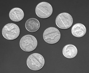
We will use the gradient to detect edges in an image. Let us start importing an image
from PIL import Image

coins = Image.open("coins.png")
We transform it into a numpy array
a = np.asarray(coins,dtype=np.float64)
plt.imshow(a,cmap='gray')
plt.show()

Now, we compute the gradient and its norm and plot the latter
py, px = np.gradient(a)
gr = np.sqrt(px**2+py**2)

plt.imshow(gr,cmap='gray')
plt.colorbar()
plt.show()

Finally we make zero all the values under some threshold and plot it again
b = gr > 50
plt.imshow(b*gr,cmap='gray')
plt.show()

- Compute the divergence of $\mathbb{f}(x,y)=(f_1(x,y),f_2(x,y))=(x^2+y^2,x^2-y^2)$ in $[-2,2]\times[-2,2]$ using the outputs of
gradientfor the functions $f_1$ y $f_2$, withhx = 0.1andhy = 0.1. Plot $\mathbb{f}$ y $\text{div} (\mathbb{f})$ in the same figure. - A boundary effect may be noticed in these plots due to the bad approximation of the divergence on these points. Remake the plots above restricting the set to $[-2+h_x,2-h_x]\times[-2+h_y,2-h_y]$.
- Compute the global relative errors of the approximation in both sets using
np.linalg.norm.
%run Exercise5


%run Exercise6
