Introduction to digital image processing using Python
Contents
Digital images
An image may be defined as a two-dimensional function $f(x,y)$, where $x$ and $y$ are spatial coordinates, and the value of $f$ at any pair of coordinates $(x,y)$ is called the intensity of the image at that point. For a gray-range image, the intensity is given by just one value (one channel). For color images, the intensity is a 3D vector (three channels), usually distributed in the order RGB.
An image may be regarded as continuous with respect to $x$ and $y$, and also in intensity (analog image). Or as a discrete function defined on a discrete domain (digital image). Both viewpoints are useful for image processing.
Converting an analog image to digital form requires both the coordinates and the intensity to be digitized. Digitizing the coordinates is called sampling, while digitizing the intensity is referred to as quantization. Thus, when all this quantities are discrete, we call the image a digital image.
The opposite operation, converting from digital to analog, is also possible and called interpolation.
Coordinate conventions
The result of sampling and quantization is a matrix of real numbers. The size of the image is the number of rows by the number of columns, $M\times N$. The indexation of the image in Python follows the usual convention:
Python modules
To install OpenCV in Anaconda python, run in terminal
$ conda install -c conda-forge opencv
Now you can import it with the other modules
import cv2 as cv                  # open vision library OpenCV
import numpy as np                # Numerical Python
import matplotlib.pyplot as plt   # Python plotting
Reading, displaying and writing images
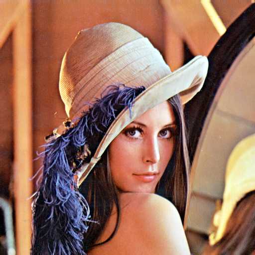
Python supports most usual image formats. Let us load the lena.jpg image
a1 = cv.imread('lena.jpg')
It is a BGR image. We swap channels R and B to have an RGB image
a2 = cv.cvtColor(a1, cv.COLOR_BGR2RGB)
The usual data type of an image is uint8, i.e. 8-bit unsigned integer. This gives $2^8 = 256$ intensity values which are distributed in the interval $[0,255]$. We'll comment on data types later on.
The variable a2 is a numpy array.
print(type(a2))
It has 512 rows, 512 columns and 3 layers.
print(a2.shape)
And its elementes are unsigned integers of 8 bits.
dt = np.dtype(a2[0,0,0])
print(dt.name)
To show the image
plt.figure()
plt.imshow(a2)
plt.show()

For converting to other formats, in this case to a gray scale image
a3 = cv.imread('lena.jpg',cv.IMREAD_GRAYSCALE)
plt.figure()
plt.imshow(a3, cmap='gray')
plt.show()

For writting to disk:
image = cv.imwrite('lena_gray.tif', a3)
Image types and conversions
There are three main types of images:
- Intensity image is a data matrix whose values have been scaled to represent intensities. When the elements of an intensity image are of class
uint8or classuint16, they have integer values in the range $[0,255]$ and $[0,65535]$, respectively. If the image is of classfloat32, the values are single-precission floating-point numbers. They are usually scaled in the range $[0,1]$, although it is not rare to use the sclae $[0,255]$ too. - Binary image is a black and white image. Each pixel has one logical value, $0$ or $1$.
- Color image is like intensity image but with three chanels, i.e. to each pixel corresponds three intensity values (RGB) instead of one.
When performing mathematical transformations of images we often need the image to be of double type. But when reading and writing we save space by using integer codification. We use the following commands
a4 = a3.astype(np.float32)
This command converts the uint8 matrix into a float32 matrix.
a5 = a4.astype(np.uint8)
image = cv.imwrite('lena_gray2.tif', a5)
This command first converts float32 numpy array a into a uint8 numpy array
The second command saves the image.
Once we have the image defined as a float32 matrix, we may start working with it (processing).
Example.
We are going to
- extract a part of the image by index restriction,
- make a plot,
- save the result.
We start with the extraction.
a = np.copy(a4)
Lena_eye=a[251:283,317:349]
The, the plotting
plt.figure()

plt.subplot(121)
plt.imshow(a,cmap='gray',interpolation='none')
plt.title('Lena'),plt.axis('off')

plt.subplot(122)
plt.imshow(Lena_eye,cmap='gray',interpolation='none')
plt.title("Right Lena's eye"),plt.axis('off')

plt.show()

And finish saving
Lena_eye = Lena_eye.astype(np.uint8)
image = cv.imwrite('LenaEye.jpg', Lena_eye)
Exercises
Write a function with
input: an image of any class and some ranges for its $(x,y)$ pixels.
output: the matrix (
float32) corresponding to the original image restricted to the given indices, and a figure of it.
Apply the function to extract the cameraman's head from cameraman.tif.
%run Exercise1.py

Masks are geometric filters on an image. For instance, if we want to extract a region of an image, we may do it by multiplying the matrix of the original image by a matrix of equal size containing $1's$ in the region we want to keep and $0's$ otherwise. In this exercise we extract a circular region of the image lena_gray_512.tif of radious 150. Follow these steps:
- Read the image and convert it to double.
- Create a matrix of the same dimensions filled with zeros.
- Modify the above matrix to contain $1's$ in a circle of radious 150, i.e. if $(j-c_x)^2+(i-c_y)^2<150^2$, where $(c_x,c_y)$ is the center of the image.
- Multiply the image by the mask (they are matrices!)
- Show the result.
When multiplying by zero, you set to black the pixels out of the circle. Modify the program to make visible those pixels with half the intensity.
%run Exercise2.py

Linear degradation is the well known effect of darkening an image vertically (or horizontally). We may do this with a mask which is constant by columns but take decreasing values in rows, from 1 in the first row to zero in the last.
Construct such matrix and apply it to Lena's image. Save the resulting image to a file.
Hint: you may use loops and if's. But vetorizing saves execution time. Explore the commands np.linspace to make the degradation and numpy.tile to construct a repited (tiled) matrix from the linspace vector output.
%run Exercise3.py

If you open the book cited in the References at page 13, you will see the functions, methods and attributes defined for the module Image of PIL, such as crop, getextrema, getpixel, histogram, resize, or rotate.
%run Exercise4.py

%run Exercise5.py

%run Exercise6.py

%run Exercise7.py
