Numerical integration
Contents
Quadrature formulas
Numerical integration or quadrature formulae have the form:
$$ \int_{a}^{b}f(x)dx\approx \omega_{0}\;f(x_{0})+\omega_{1}\;f(x_{1})+\cdots +\omega_{n}\;f(x_{n}) $$where $x_{0},x_{1},...,x_{n}$ (nodes) are $n+1$ different points in the interval $[a,b]$ and $\omega_{0},\omega_{1},\ldots ,\omega_{n}$ (weights) are real numbers.
Interpolatory quadrature formulas
If $P_{n}$ is the polynomial interpolation function for $f$ in the nodes $x_{0},x_{1},...,x_{n} \in \left[ a,b\right]$ and
$$ \int_{a}^{b}f(x)dx\approx \int_{a}^{b}P_n(x)dx=\omega_{0}\,f(x_{0})+\omega_{1}\,f(x_{1})+\cdots +\omega_{n}\,f(x_{n}) $$this is called an interpolatory quadrature formula.
Simple and composite quadrature formulas
Quadrature formulas are called simple if the approximation takes place in the whole interval $(a,b)$, and composite if, before the application of the formula, we split the interval $(a, b)$ in a given number, $n$, of subintervals.
Degree of precision
The degree of precision is used for simple quadrature formulas. A quadrature formula has degree of precision $r$ if the rule is exact for
$$ f\left( x\right) =1,\quad f\left( x\right) =x,\quad f\left( x\right) =x^{2},...,f\left( x\right) =x^{r}$$and it is not for $f\left( x\right) =x^{r+1}$
Simple Newton-Cotes formulas
They are interpolatory quadrature formulas where the nodes are equispaced within the interval. There are two types of Newton-Cotes formulas
- Closed formulas. The integration limits $a$ and $b$ are nodes.
- Open formulas. The integration limits $a$ and $b$ are not nodes.
Let us compute first the exact integral
%matplotlib inline
We import the modules numpy y sympy
import numpy as np
import sympy as sym
And the exact value of
$$ \int_0^3 e^x \,dx$$is
x = sym.Symbol('x', real=True)
f = sym.exp(x)
I_exacta = sym.integrate(f,(x,0,3))
print(I_exacta)
We also can express it as
I_exacta = float(I_exacta)
print(I_exacta)
Middle point rule
The Middle point rule is
$$\int_{a}^{b}f(x)dx\approx (b-a)\;f\left( \frac{a+b}{2}\right)$$The formula can be generated substituting the function inside the integral by the zero degree polynomial that passes throught the point of the curve in the center of the $[a,b]$ interval; that is, the horizontal line that passes throught the middle point of the function. Geometrically, we are computing the area of a rectangle.
Write a middle_point(f,a,b) function whose input are the function f and the boundaries of the integration interval a and b, and the output, the approximate value of the integral using the Middle Point rule. Compute the integral
Print the exact value (calculated above) and the approximate value.
%run Exercise1.py

Trapezoidal rule
The simple Trapezoidal rule is
$$\int_{a}^{b}f(x)dx\approx \frac{b-a}{2}\;\left( f\left( a\right) +f\left( b\right) \right)$$The formula can be generated substituting the function inside the integral by the one degree polynomial that passes throught the points of the curve in the boundaries of the $[a,b]$ interval; that is, the line that passes throught two boundary points of the function in the interval. Geometrically, we are computing the area of a trapezoid.
Write a trapez(f,a,b) function whose input are the function f and the boundaries of the integration interval a and b, and the output, the approximate value of the integral using the Trapezoidal rule. Compute the integral
Print the exact value and the approximate value.
%run Exercise2.py

Simpson rule
La fórmula de Simpson simple es
$$\int_{a}^{b}f(x)dx\approx \frac{b-a}{6}\;\left( f\left( a\right) +4\;f\left( \frac{a+b}{2}\right) +f\left( b\right) \right)$$Usar la fórmula de Simpson para integrar una función en un intervalo, equivale a sustituir, dentro de la integral, la función a integrar por el polinomio de interpolación de grado dos, que pasa por los puntos de la función de los extremos y el punto medio del intervalo. Es decir, sustituimos la función por una parábola e integramos.
The formula can be generated substituting the function inside the integral by the two degree polynomial that passes throught three points of the curve in the boundaries and the middle point of the $[a,b]$ interval; that is, the parabola that passes throught these three pointsin the interval. Geometrically, we are computing the area under the parabola.
%run Exercise3.py

Composite Newton-Cotes formulas
A way to decrease the error is to increase the number of nodes using the composite rules. They are obtained splitting the interval $\left[ a,b\right] $ in $n$ subintervals and using, for each of this subintervals, the simple quadrature rule.
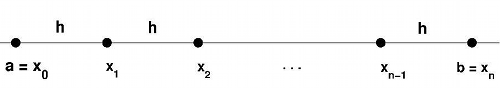
If we divide the interval $\left[ a,b\right] $ into $n$ subintervals of equal length using the nodes $x_{0},x_{1},...,x_{n}$,
the length of a subinterval is
$$h=\frac{b-a}{n}$$the nodes are
$$x_i=a+i\,h \quad i=0,1,\ldots,n$$and the middle point of a subinterval is
$$\bar x_i =\frac{x_{i-1}+x_i}{2}$$then, the composite formulas can be written:
Composite Middle Point rule
$$ \int_a^b f dx \approx h\sum_{i=1}^{n}f(\bar x_i)$$Write a comp_middle_point(f,a,b,n) function whose input are the function f and the boundaries of the integration interval a and b, and n the number of subintervals, and the output, the approximate value of the integral using the composite Middle Point rule. Compute, with n = 5 subintervals the integral
Print the exact value and the approximate value.
%run Exercise4.py

Composite Trapezoidal rule
$$ \int_a^b f dx \approx \frac{h}{2}(f(a)+f(b))+h\sum_{i=1}^{n-1}f(x_i)$$Write a comp_trapz(f,a,b,n) function whose input are the function f and the boundaries of the integration interval a and b and n the number of subintervals, and the output, the approximate value of the integral using the composite Trapezoidal rule. Compute, with n = 4 subintervals the integral
Print the exact value and the approximate value.
%run Exercise5.py

Composite Simpson rule
$$ \int_a^b f dx \approx \frac{h}{6}\sum_{i=1}^{n}\left(f(x_{i-1})+4f(\bar x_i)+f(x_i)\right)) $$Write a comp_simpson(f,a,b,n) function whose input are the function f and the boundaries of the integration interval a and b and n the number of subintervals, and the output, the approximate value of the integral using the composite Simpson rule. Compute, with n = 4 subintervals the integral
Print the exact value and the approximate value.
%run Exercise6.py

Gaussian quadrature formulas
In the quadrature formula
$$ \int_{a}^{b}f(x)dx\approx \omega_{0}\,f(x_{0})+\omega_{1}\,f(x_{1})+\cdots +\omega_{n}\,f(x_{n}) $$Is is possible to compute the weights $\omega_i$ and the nodes $x_i$ so the precision of the formula is maximum? Yes, but then, the nodos are not equispaced.
If we have $n$ nodes in $[a,b]=[-1,1]$ the weights and the nodes are
For instance, the gaussian formula with one node
$$ \int_{-1}^{1}f(x)dx\approx 2\;f(0) $$that it is the same as the Middle Point rule. For two nodes
$$ \int_{-1}^{1}f(x)\;dx\approx f(-0.577350)+f(0.577350) $$For three nodes $$ \int_{-1}^{1}f(x)\;dx\approx 0.555556\;f(-0.774597)+0.8888889\;f(0)+ 0.555556\;f(0.774597) $$
And so on.
This formulas can be generalized for any interval $[a,b]$ changing $x_i$ with $y_i$ following the
$$y_i=\frac{b-a}{2}x_i+\frac{a+b}{2}$$And then, the quadrature formula is
$$ \int_{a}^{b}f(x)\,dx\approx\frac{b-a}{2}\left( \omega_{0}\;f(y_{0})+\omega_{1}\;f(y_{1})+\cdots +\omega_{n}\;f(y_{n})\right) $$Write a gauss(f,a,b,n) function whose input are the function f and the boundaries of the integration interval a and b and n the number of interpolation points, and the output, the approximate value of the integral using the gaussian formula. Compute, with n = 1, n = 2 and n = 3 nodes the integral
Print the exact value and the approximate value.
%run Exercise7.py


Numerical integration with python commands
The module scipy.integrate contains different integrating functions. For instance, the function quad
import scipy.integrate as integrate

f = lambda x : np.exp(x)
a = 0.; b = 3;

I = integrate.quad(f,a,b)

print 'The approximate value is %f' % (I[0])
print 'The exact value is       %f' % (I_exacta)