Introduction to Matlab

This tour introduces the basic notions of programming with Matlab.

M-file scripts
M-file functions
Inline functions
Loops
Conditionals
References

M-file scripts

A script file is an external file that contains a sequence of MATLAB statements.

Script files have a filename extension .m and are often called M-files.

M-files can be scripts that simply execute a series of MATLAB statements, or they can be functions that can accept arguments and can produce one or more outputs.

Here are two simple scripts.

Example 1.1 Find the solution of the following system of equations

\[ x+2y+3z=1,\quad 3x+3y+4z=1,\quad 2x+3y+3z=2.\]

Solution: We write the m-file example1.m containing the following commands, and execute it in the command window of Matlab simply by typing

>> example1

clear all
A=[1 2 3; 3 3 4; 2 3 3];
b= [1;1;2];
x=A\b

When execution completes, the variables (\(A\), \(b\), and \(x\)) remain in the workspace. To see a listing of them, enter whos at the command prompt.

whos

  Name      Size            Bytes  Class     Attributes

  A         3x3                72  double              
  b         3x1                24  double              
  x         3x1                24  double

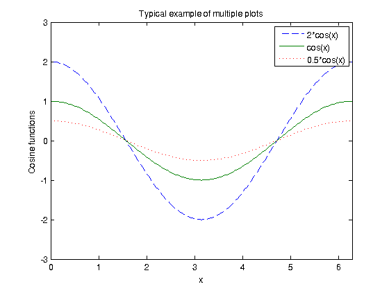
Example 1.2 Plot the following cosine functions, \(y1 = 2 \cos(x)\), \(y2 = \cos(x)\), and \(y3 = 0.5\cos(x)\), in the interval \(0 \leq x \leq 2\pi\). Here we write the commands in the file example2.m

x = 0:pi/100:2*pi;
y1 = 2*cos(x);
y2 = cos(x);
y3 = 0.5*cos(x);
plot(x,y1,'--',x,y2,'-',x,y3,':')
xlabel(' x ')
ylabel('Cosine functions')
legend('2*cos(x)','cos(x)','0.5*cos(x)')
title('Typical example of multiple plots')
axis([0 2*pi -3 3])

Exercise 1.1 Write a program (exercise1_1.m) to find the roots of the second order polynomial \(ax^2 +bx +c\), for any given numbers \(a,~b\) and \(c\), defining them as \(a=1,~b=1,~c=3\).

M-file functions

Functions are programs (or routines) that accept input arguments and return output arguments.

Each M-file function has its own area of workspace, separated from the MATLAB base workspace.

The name of the script function must coincide with the name of the function.

The first line of a function M-file starts with the keyword function. It gives the function name and order of arguments.

These simple functions show the basic parts of an M-file.

Omit the % in your script. We have to write them here for technical reasons.

Example 1.3 Script function f.m, for computing the square of a number.

%function z=f(x)
%z=x^ 2;

f(2)

ans =

     4

Example 1.4 Script function measures_spere.m, for computing the area and volume of a sphere of radious R.

%function [area,volume]=measures_sphere(R)
%area=4*pi*R.^ 2;
%volume=(4/3)*pi*R.^3;

R=[0:0.1:0.5];
[a,v]=measures_sphere(R)

a =

         0    0.1257    0.5027    1.1310    2.0106    3.1416


v =

         0    0.0042    0.0335    0.1131    0.2681    0.5236

Exercise 1.2 Write a function (exercise1_2.m) to find the roots of the second order polynomial of Exercise 1.1, but now with the parameters a,b,c passed as arguments.

Inline functions

We also may define simple functions inside a script without using M-files. It uses the sintaxis f=@(x) expression of x;

For instance

Area=@(R) 4*pi*R.^ 2;
Area(R)

ans =

         0    0.1257    0.5027    1.1310    2.0106    3.1416

Loops

Loops in Matlab may be built by for and while statements. The for estatement has the syntaxis

% for i=vector
%	set of instructions
% end
% where vector is given, usually, as vector=first:increment:last
% If increment=1, we write vector=first:last

Example 1.5

Sum=0;Factorial=1;
for k=1:5
  Sum=Sum+k;
  Factorial=Factorial*k;
end
[Sum,Factorial]

ans =

    15   120

Example 1.6 Two ways to defining a uniform mesh of the interval (0,1).

The first is more efficient and uses what is called "vectorization".

In Matlab, vectorization often saves execution time. The command tic-toc measures time execution.

dx=0.001;
tic
x=[0:dx:1];
toc
tic
X(1)=0;
for k=2:(1/dx)+1
  X(k)=(k-1)*dx;
end
toc
disp(['norm(x-X) = ', num2str(norm(x-X))])	% norm(y) -> Euclidian norm of y, i.e. sqrt(sum(y_i^2))
disp(['machine epsilon = ', num2str(eps)])

Elapsed time is 0.001067 seconds.
Elapsed time is 0.002951 seconds.
norm(x-X) = 1.1749e-15
machine epsilon = 2.2204e-16

Observe that \(\mbox{norm}(x-X)=0\) would tell us that \(x=X\) (in the sense of floating-point representation). However, this is not the case due to accumulation of rounding errors

for loops may be nested:

for i=1:3
    for j=1:2
        A(i,j)=i*j;
    end
end
A

A =

     1     2     3
     2     4     4
     3     6     3

Exercise 1.3 Write a script (exercise1_3.m) to compute the approximated solution to the differential equation \[ x'(t)= a*x(t) \quad\mbox{for}\quad t \in (0,1),\] with the initial datum \(x(0)=1\). Then, compare it with the exact solution \(y(t)=\exp(a*t)\).

Follow these steps:

Define \(a=-0.5\), \(t_{\rm end}=10\).
Define a partition, \(t\), of \((0,1)\) with \(dt=0.01\).
Allocate the solution in a vector of zeros (find the size) and define the initial datum x(1)=1.
Make a for loop to compute \(x(k+1)=x(k)+dt*a*x(k)\).
Define y as an inline function.
Compute the relative error between x and y at \(t=t_{\rm end}\);
Plot \(x\) and \(y\) in the same window.

A while loop executes a group of statements for as long as the expression controlling the loop is true. The syntax is similar to that of for:

% while expression
%	statements
% end

while and for loops may be nested:

t=0;T=1;x=0;
while t<T
    t=t+0.1;
        for i=1:10
            x=x+(i/t);
        end
end
x

x =

   1.6609e+03

Conditionals

Conditional statement if has, in its simplest version, the syntax

% if expression
%   statements
% end

Example 1.7

for k=1:5
    if k^3>30
        disp('k is larger than 30')
    end
end

k is larger than 30
k is larger than 30

If there are several options then we use

% if expression1
%   statements1
% elseif statements2
%   statements2
% else
%   statements3
% end

Example 1.8 Suppose we want to write a funtion to add a variable amount of numbers. Then we may define the output depending on the number of input arguments.

%uncomment the following when writting the m-file
%function d = addme(a,b,c)
%
%if nargin==3
%    d=a+b+c;
%elseif nargin==2
%    d=a+b;
%else
%     d=a;
%end

d1=addme(1,5);
fprintf('d=%d\n',d1)
d2=addme(1,5,3);
fprintf('d=%d\n',d2)

d=6
d=9

The break command terminates the execution of a for or while loop. When a break statement is encountered, execution continues with the next statement outside the loop:

Example 1.9

for i=1:5
    if i>3
        break
    end
    i
end

In nested loops, break exits only from the inner-most loop that contains it:

Example 1.10

for i=1:5
    for j=1:3
        if i>3 | j==2
            break
        end
    end
     [i j]
end

Exercise 1.4 Modify the script of Exercise 1.3 (and save it as exercise1_4.m) to compute the approximated solution to the same differential equation but introducing a sttoping criterium based on the absolute difference between two succesive iterations. Then, compare it again with the exact solution \(y(t)=\exp(a*t)\).

Follow these (additional) steps:

Define the absolute difference between two iterations, \[ad=\left| x(k+1)-x(k) \right| .\]
Define a tolerance tol=1.e-4 for the stopping criterium.
Use either a combination of for and if to implement the stopping, or a simple while (changing suitably the for loop of Exercise 1.3)

References

We recall here some basic Matlab commands the reader should already know, see Intro to Matlab

A longer introduction to Matlab may be found in Mathwork's Getting Started with Matlab