Introduction to image processing

Digital images
Coordinate conventions
Reading, displaying and writing images
Image types and coversions
Exercises

In this series of labs we shall illustrate several of the numerical methods introduced in the theory lectures by image processing applications. We introduce in this lab some of the fundamental features of image representation and manipulation with Matlab.

Digital images

An image may be defined as a two-dimensional function \(f(x,y)\), where \(x\) and \(y\) are spatial coordinates, and the value of \(f\) at any pair of coordinates \((x,y)\) is called the intensity of the image at that point.

An image may be continuous with respect to \(x\) and \(y\), and also in intensity (analog image). Converting such an image to digital form requires that the coordinates and the intensity be digitized. Digitizing the coordinates is called sampling, while digitizing the intensity is referred to as quantization. Thus, when all this quantities are discrete, we call the image a digital image.

Coordinate conventions

The result of sampling and quantization is a matrix of real numbers. The size of the image is the number of rows by the number of columns, \(M\times N\). The indexation of the image follows the following conventions: \[{\rm Usual}\longrightarrow \left( \begin{array}{ccccc} a(0,0) & a(0,1) & \ldots & a(0,N-2) & a(0,N-1)\\ a(1,0) & a(1,1) & \ldots & a(1,N-2) & a(1,N-1) \\ \ldots & \ldots & \ldots & \ldots & \ldots \\ a(M-1,0) & a(M-1,1) & \ldots & a(M-1,N-2) & a(M-1,N-1) \end{array} \right)\ \qquad\qquad \left( \begin{array}{ccccc} a(1,1) & a(1,2) & \ldots & a(1,N-1) & a(1,N)\\ a(2,1) & a(2,2) & \ldots & a(2,N-1) & a(2,N) \\ \ldots & \ldots & \ldots & \ldots & \ldots \\ a(M,1) & a(M,2) & \ldots & a(M,N-1) & a(M,N) \end{array} \right) \longleftarrow {\rm Matlab }\]

Reading, displaying and writing images

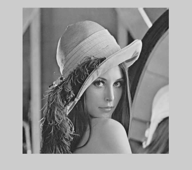
Matlab supports most usual image formats. The reading syntax is

a=imread('lena_gray_512.tif');
whos

  Name        Size              Bytes  Class    Attributes

  a         512x512            262144  uint8

The usual data type of an image is uint8, i.e. 8-bit integer type. This gives a range of \([0,255]\) for each pixel. We'll comment on data types later on.

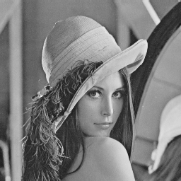
For visualizing we may use imshow, which has several options

figure,imshow(a)
figure,imshow(a,'InitialMagnification',50,'Border','tight')

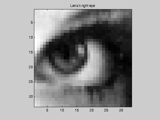
Since the image is now a matrix, we may extract portions of it. Commands image and imagesc are other more flexible ways to visualize images

lena_eye=a(252:284,318:350);
figure,imagesc(lena_eye)
colormap(gray)
axis image        % Set aspect ratio to obtain square pixels
title('Lena''s right eye')

And we write it to the working directory using imwrite

imwrite(lena_eye,'lena_eye.png');

The following command displays image information

imfinfo('lena_gray_512.tif')

ans = 

                     Filename: [1x70 char]
                  FileModDate: '28-ago-2008 15:03:30'
                     FileSize: 262598
                       Format: 'tif'
                FormatVersion: []
                        Width: 512
                       Height: 512
                     BitDepth: 8
                    ColorType: 'grayscale'
              FormatSignature: [73 73 42 0]
                    ByteOrder: 'little-endian'
               NewSubFileType: 0
                BitsPerSample: 8
                  Compression: 'Uncompressed'
    PhotometricInterpretation: 'BlackIsZero'
                 StripOffsets: [32x1 double]
              SamplesPerPixel: 1
                 RowsPerStrip: 16
              StripByteCounts: [32x1 double]
                  XResolution: 72
                  YResolution: 72
               ResolutionUnit: 'Inch'
                     Colormap: []
          PlanarConfiguration: 'Chunky'
                    TileWidth: []
                   TileLength: []
                  TileOffsets: []
               TileByteCounts: []
                  Orientation: 1
                    FillOrder: 1
             GrayResponseUnit: 0.0100
               MaxSampleValue: 255
               MinSampleValue: 0
                 Thresholding: 1
                       Offset: 262152

Image types and coversions

There are three main image types

Intensity image is a data matrix whose values have been scaled to represent intensities.When the elements of an intensity image are of class uint8 or class uint16, they have integer values in the range \([0,255]\) and \([0,65535]\), respectively. If the image is of class double, the values are floating-point numbers. Values of scaled, class double intensity images are in the range \([0,1]\) by convention.
Binary image is a black and white image. Each pixel has one logical value, \(0\) or \(1\).
Color image is like intensity image but with three chanels, i.e. to each pixel corresponds three intensity values (RGB) instead of one.

When performing mathematical transformations of images we often need the image to be of double type. But when reading and writing we save space by using integer codification. We use the following commands

im2uint8: from any type to uint8 class,
im2double: from any type to double (rescaled),
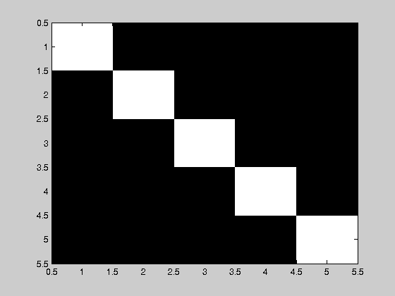
im2bw: from any type to logical,
rgb2gray: RGB color to gray.

a1=lena_eye(1:5,1:5)
a2=im2double(a1)
b1=eye(5);
b2=im2bw(b1);
whos a1 a2 b1 b2
imagesc(b2)

a1 =

  186  188  193  195  197
  186  187  193  189  194
  190  186  188  186  192
  192  190  191  190  193
  190  187  189  192  192


a2 =

    0.7294    0.7373    0.7569    0.7647    0.7725
    0.7294    0.7333    0.7569    0.7412    0.7608
    0.7451    0.7294    0.7373    0.7294    0.7529
    0.7529    0.7451    0.7490    0.7451    0.7569
    0.7451    0.7333    0.7412    0.7529    0.7529

  Name      Size            Bytes  Class      Attributes

  a1        5x5                25  uint8                
  a2        5x5               200  double               
  b1        5x5               200  double               
  b2        5x5                25  logical

Exercises

exercise 1 Make a function (exercise3_1.m) with

input: one image of any class and some ranges for its \((x,y)\) pixels. Hint: store them in a single vector.
output: the matrix (double class) corresponding to the original image restricted to the given indices, and a figure of it.

Apply it to select the head of the cameraman of cameraman.tif.

Exercise 2 Masks are geometric filters on an image. For instance, if we want to select a region of an image, we may do it by multiplying the matrix of the original image by a matrix of equal size containing \(1's\) in the region we may to keep and \(0's\) otherwise. In this exercise we select a circular region of the image lena_gray_512.tif of radious 150. Follow these steps (file exercise3_2.m)

Read the image and convert it to double.
Create a matrix of the same dimensions filled with zeros.
Modify the above matrix to contain \(1's\) in a circle of radious 150, ie if \((i-c_x)^2+(j-c_y)^2<150^2\), where \((c_x,c_y)\) is the center of the image.
Multiply the image by the mask (they are matrices!)
Show the result.

When multiplying by zero, you set to black the pixels out of the circle. Modify the program to make visible those pixels with half the intensity.

Exercise 3 Linear degradation is the well known effect of darkening an image vertically (or horizontally). We may do this with a mask which is constant by columns but take decreasing values in rows, from 1 in the first row to zero in the last. Construct such matrix and apply it to Lena's image (file exercise3_3.m).

Hint: you may use loops and if's. But vetorizing saves execution time. Explore the Matlab commands linspace to make the degradation and repmat to construct a repited matrix (rep-mat) from the linspace vector output.