Zeros of nonlinear functions
Contenidos
%
Solutions to equations
A real scalar equation is an expression of the form
\[f(x)=0,\]
where \(f:\Omega\subset\mathbb{R}\rightarrow\mathbb{R}\) is a function.
Any number, \(\alpha\), satisfying \(f(\alpha)=0\) is said to be a solution of the equation or a zero of \(f\). If \(f\) is a polynomial the their zeros are called roots.
Example 4.1 Compute graphically an approximation to the solutions of
\[x^3-2x^2+1=0.\]
f=@(x)x.^3-2*x.^2+1;
x=linspace(-1,2);
plot(x,f(x))
hold on
plot([-1 2],[0,0],'k-') % plot of X axis
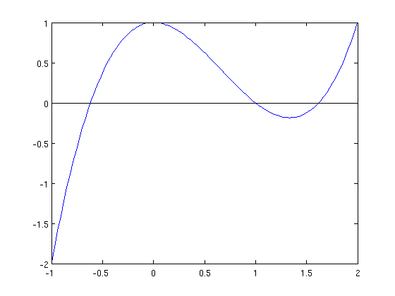
We see that there are three solutions (intersections with \(X\) axis). They are, approximately, \(x\simeq -0.6\), \(x\simeq 0.9\) and \(x\simeq 1.6\)
Separation of zeros
From the plot above, we see that we may separate the zeroes of \(f\) in intervals satisfying the conditions of Bolzano's theorem:
Let \(f:[a,b]\rightarrow\mathbb{R}\) be a continuous function with \(f(a)f(b)<0\). Then, there exists at least one zero of \(f\) in \([a,b]\).
So we seek for intervals where \(f\) changes its sign.
In addition, if the function is increasing or decreasing, then there only can exist a unique zero.
In our example, there are three intervals satisfying these conditions:
\[ [-1,-0.1]\quad [0.5,1.1] \quad [1.5,2] \]
Bisection method
The Bisection method works for a continuous funtion \(f\) defined on a bounded interval, \([a,b]\), where Bolzano's theorem conditions are satisfied. The separation condition is not necessary, but in case that several zeros are located in \([a,b]\), the Bisection method will approximate only one.
Algorithm
- --Let \(a_1=a\), \(b_1=b\).
- --While \(k\leq MaxIter\) and \( Error > BoundError)\)
- ---------Compute the middle point \(x_k=\frac{a_k+b_k}{2}\) and evaluate \(f(x_k)\).
- ---------if \(f(a_k)f(x_k)<0\) then \( a_{k+1}=a_{k},\quad b_{k+1}=x_k,\)
- --------on the contrary, \( a_{k+1}=x_{k},\quad b_{k+1}=b_k.\)
- --------Compute Error
Observe that
- The approximation is given by any point of the interval. Usually, one takes one of the extremes.
- The maximum error is the length of the interval.
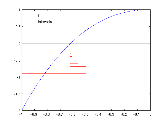
In the following plot we draw the sequence of intervals (in red) to compute the first zero of \(f\).
bisection_draw
Exercise 4.1 Write a script bisection1.m for the inline function \(f\) given in the Example 4.1, and for generic intervals \([a,b]\). Set the maximum number of iterations to \(n=20\) and do not use any stopping criterium. Provide the output solution using the Matlab command fprintf('x = %f',x), where x is the approximate solution.
If we use the function and intervals of Example 4.1 with 20 iterations we get
a=-1;b=-0.1;
bisection1;
x = -0.618034
a=0.5;b=1.1;
bisection1;
x = 1.000000
a=1.5;b=2;
bisection1;
x = 1.618034
Stopping criteria
Since the sequence \(\{x_k\}\) such that \(x_k\rightarrow \alpha\), with \(f(\alpha)=0\) is, in general, infinite, we must introduce some stopping criterium to stop the algorithm when the approximation is good enough.
Stopping criteria are based on:
- Absolute error \( \left| x_k-x_{k-1}\right| <\epsilon\).
- Relative error \( \frac{\left|x_k-x_{k-1}\right|}{\left|x_k\right|}<\epsilon\).
- Residual \( \left|f(x_k)\right|<\epsilon\).
Exercise 4.2 We are going to
- Modify the script bisection1.m to add the absolute value stopping criterium. Write it in a script called bisection2.m
- Transform bisection2.m into a Matlab function with
- Input arguments: \(f\), \(a\), \(b\) and the absolute error bound \(E_a=0.001\).
- Output arguments: approximate solution and number of performed iterations.
Ea=0.001;a=-1;b=-0.1;
[x,n]=bisection2(f,a,b,Ea);
fprintf('x = %f   n=%d ',x,n)
x = -0.617676 n=10
a=0.5;b=1.1;
[x,n]=bisection2(f,a,b,Ea);
fprintf('x = %f   n=%d ',x,n)
x = 0.999805 n=10
a=1.5;b=2;
[x,n]=bisection2(f,a,b,Ea);
fprintf('x = %f   n=%d ',x,n)
x = 1.618164 n=9
Newton-Raphson method
We use this method when the exact differential may be computed.
In each step, the function \(f\) is replaced by its tangent line, \(t\), in the point \(x_k\), and the corresponding zero is computed as an approximation to the true solution.
Algorithm
- --Let \(x_0\) be an initial guess.
- --While \(k\leq MaxIter\) and \( Error > BoundError)\)
- ---------Compute \[x_k=x_{k-1}-\frac{f(x_{k-1})}{f'(x_{k-1})}\]
- ---------Compute Error
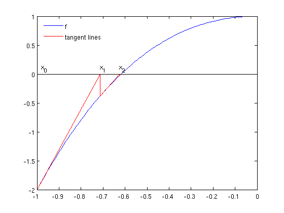
In the plot, we see the sequence of tangent lines (in red) for computing the first zero. The inital guess iso \(x_0=-1\).
newton_draw
Exercise 4.3 Write a function newton.m with input arguments:
- \(f\) and its differential \(df\) given as inline functions,
- the initial guess \( \(x_0\),
- The relative error bound \(E_a=0.001\).
And with output arguments:
- Approximate solution.
- Number of performed iterations.
Compare with the results of Exercise 4.2.
If we use the intervals and function of Example 2.1:
f=@(x)x.^3-2*x.^2+1;           % function
df=@(x)3*x.^2-4*x;             % derivative
Ea=0.001;x0=-1;                % data
[x,n]=newton(f,df,x0,Ea);      % evaluation
fprintf('x = %f   n=%d ',x,n); % printing
x = -0.618034 n=4
x0=0.5;
[x,n]=newton(f,df,x0,Ea);
fprintf('x = %f   n=%d ',x,n);
Exact solution achieved
x = 1.000000   n=1
x0=1.5;
[x,n]=newton(f,df,x0,Ea);
fprintf('x = %f   n=%d ',x,n);
x = 1.618034 n=4
Secant method
It is the most important variant of Netwon-Raphson method. We replace the tangent line by the secant.
The main inconvinient of Newton-Raphson method is that we need to compute in advance \(f'(x)\).
In the Secant method we approximate \(f'(x)\) by finite differences: \[f'(x_{k-1})=\frac{f(x_{k-1})-f(x_{k-2})}{x_{k-1}-x_{k-2}}.\]
In counterpart, we need two initial guesses, \(x_0\) y \(x_1\) for the first iteration: \[ x_k= x_{k-1} -f( x_{k-1})\frac{x_{k-1}-x_{k-2}}{f(x_{k-1})-f(x_{k-2})}.\]
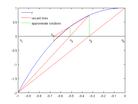
In the plot we see the sequence of secants (in red) to compute the first zero of \(f\), taking initial guesses \(x_0=0\) and \(x_1=-1\). In green, the location of the sequence of computed approximations.
secant_draw
Exercise 4.4 Transform newton.m into secant.m by introducing suitable changes.
If we use the intervals and function of Example 4.1:
Ea=0.001;x0=-1;x1=-0.1;
[x,n]=secant(f,x0,x1,Ea);
fprintf('x = %f   n=%d ',x,n);
x = -0.618034 n=7
x0=0.5;x1=1.1;
[x,n]=secant(f,x0,x1,Ea);
fprintf('x = %f   n=%d ',x,n);
x = 1.000000 n=4
x0=1.5;x1=2;
[x,n]=secant(f,x0,x1,Ea);
fprintf('x = %f   n=%d ',x,n);
x = 1.618031 n=5
Order of convergence
Numerical methods to compute zeroes of functions are iterative methods, i.e. a sequence \( x_0,x_1,\ldots,x_k,\ldots\) is constructed, such that \[\lim_{k\to\infty}f(x_k)=0.\]
The order of convergence of a method is related to the sequence speed of convergence with respect to \(k\).
This is a useful concept to compare different methods.
We say that \(x_k\) converges to \(\alpha\) with order of convergence \(p\) if \[ \lim_{k\to\infty}\frac{|x_k-\alpha|}{|x_{k-1}-\alpha|^p}=\lambda\neq 0 \quad\quad\quad (\mbox{Expression 1}) \] In the particular cases
- \(p=1\), we say that the order is linear \(\rightarrow\) Bisection method
- \(p=2\), we say that the order is quadratic \(\rightarrow\) Newton-Raphson method.
- \(p\in(1,2)\), we say that the order is super-linear \(\rightarrow\) Secant method \(p=1.618\).
A numerical method is said to be of order \(p\) if it defines a sequence which converges to the exact solution with order \(p\).
Exercise 4.5 Copy the functions bisection2, newton and secant, calling them bisection3.m, newton2.m and secant2.m. Then modify them by replacing the stopping criterium by just doing a fixed number of iterations, \(n\). As output, give all the approximations generated by the algorithm.
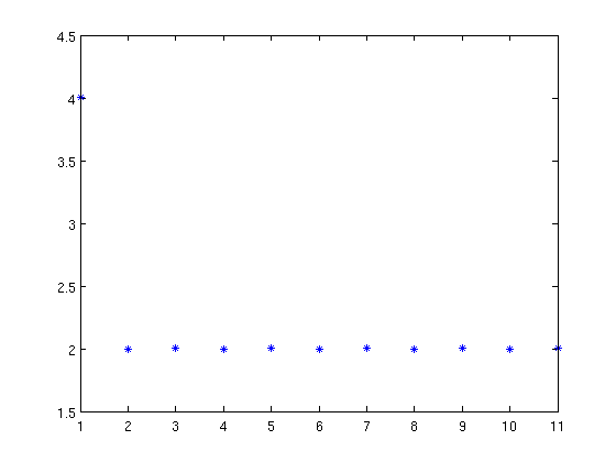
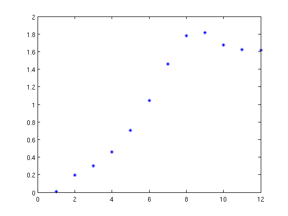
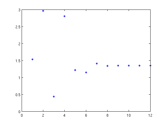
Then, use the zero \(\alpha=1\) to test the order of convergence according to the following schemes.
- Bisection, \(p=1\).
- Newton-Raphson, \(p=2\).
- Secant, \(p=1.618\).
f=@(x)x.^3-2*x.^2+1;
df=@(x)3*x.^2-4*x;
a=0.5;b=1.1;n=12;
x=bisection3(f,a,b,n);
p=1;
lambda=abs((x(1:end-1)-1)./(x(2:end)-1).^p); % Computing expression (1)
figure;plot(lambda,'*');                     % The sequence tends to a constant
x0=0.02;n=12;
x=newton2(f,df,x0,n);
p=2;
lambda=abs((x(1:end-1)-1)./(x(2:end)-1).^p);
figure;plot(lambda,'*')
x0=0.5;x1=1.5;n=12;
x=secant2(f,x0,x1,n);
p=1.618;
lambda=abs((x(1:end-1)-1)./(x(2:end)-1).^p);
figure;plot(lambda,'*')
Exact solution achieved
Matlab functions
We may compute the zeros of a function using Matlab function fzero. In its simplest form, we pass as arguments the function and an initial guess.
f=@(x)x.^3-2*x.^2+1;
x1=fzero(f,-1);
x2=fzero(f,1);
x3=fzero(f,2);
fprintf('x1 = %f,  x2 = %f, x3 = %f',x1,x2,x3);
x1 = -0.618034, x2 = 1.000000, x3 = 1.618034
Matlab uses a combination of the Bisection method, in the first iterations, to separate the zeroes, and the Secant method, to converge faster to the solution, once the zeroes are separated. More info in Mathworks-fzero
If the function is a polynomial, function roots computes all its solutions simultaneously. As input argument we give the coefficients ordered in a vector.
roots([1 -2 0 1])
ans =

    1.6180
    1.0000
   -0.6180
More info in Mathworks-roots