Interpolation and polynomial approximation
Contents
Interpolant polynomial
Problem. We are given a collection of points \((x_0,y_0),(x_1,y_1),\ldots,(x_n,y_n)\) and are asked to find a polynomial passing through all of them.
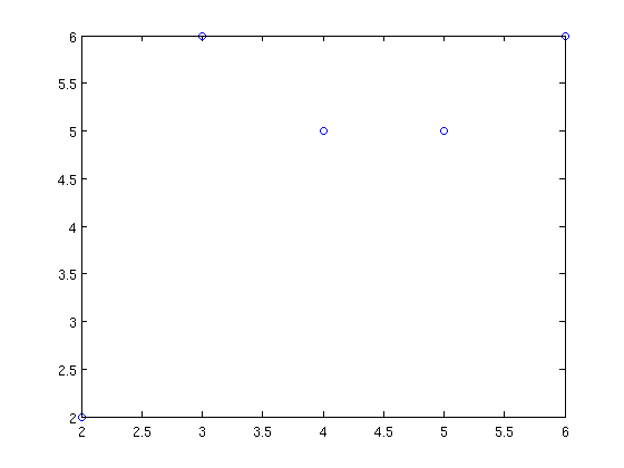
For example, take \[C=\{(2,2),(3,6),(4,5),(5,5),(6,6)\}\]
We draw the points in the plane:
x=[2,3,4,5,6];
y=[2,6,5,5,6];
plot(x,y,'o')
Solution using the Vandermonde matrix
A polynomial of degree 4 \[P_4(x)=a_0+a_1x+a_2x^2+a_3x^3+a_4x^4,\] depends on 5 unknowns, the coefficients. To determine them, we set 5 equations, corresponding to the evaluation of \(P_4\) in the 5 points of \(C\): \[ \begin{array}{lll} P_{4}(x_{0})=y_{0} & \quad & a_{0}+a_{1}x_{0}+a_{2}x_{0}^{2}+a_{3}x_{0}^{3}+a_{4}x_{0}^{4}=y_{0}\\ P_{4}(x_{1})=y_{1} & \quad & a_{0}+a_{1}x_{1}+a_{2}x_{1}^{2}+a_{3}x_{1}^{3}+a_{4}x_{1}^{4}=y_{1}\\ P_{4}(x_{2})=y_{2} & \quad & a_{0}+a_{1}x_{2}+a_{2}x_{2}^{2}+a_{3}x_{2}^{3}+a_{4}x_{2}^{4}=y_{2}\\ P_{4}(x_{3})=y_{3} & \quad & a_{3}+a_{1}x_{3}+a_{2}x_{3}^{2}+a_{3}x_{3}^{3}+a_{4}x_{3}^{4}=y_{3}\\ P_{4}(x_{4})=y_{4} & \quad & a_{0}+a_{1}x_{4}+a_{2}x_{4}^{2}+a_{3}x_{4}^{3}+a_{4}x_{4}^{4}=y_{4} \end{array} \]
which is represented in matrix form as \[ \left(\begin{array}{ccccc} 1 & x_{0} & x_{0}^{2} & x_{0}^{3} & x_{0}^{4}\\ 1 & x_{1} & x_{1}^{2} & x_{1}^{3} & x_{1}^{4}\\ 1 & x_{2} & x_{2}^{2} & x_{2}^{3} & x_{2}^{4}\\ 1 & x_{3} & x_{3}^{2} & x_{3}^{3} & x_{3}^{4}\\ 1 & x_{4} & x_{4}^{2} & x_{4}^{3} & x_{4}^{4} \end{array}\right)\left(\begin{array}{c} a_{0}\\ a_{1}\\ a_{2}\\ a_{3}\\ a_{4} \end{array}\right)=\left(\begin{array}{c} y_{0}\\ y_{1}\\ y_{2}\\ y_{3}\\ y_{4} \end{array}\right) \]
The matrix of this system is called the Matrix of Vandermonde.
Exercise 5.1.
- Write a function V=Vandermonde(x) with input: vector x, and output: Vandermonde's matrix, V.
Once we have the matrix, we may compute the coefficients of the polynomial given in the above example by solving the system.
V=Vandermonde(x)
a=V\y';
aa=a(end:-1:1)'  % trasposition and reordering, to start with the coefficient corresponding to the higher order term.
V =

           1           2           4           8          16
           1           3           9          27          81
           1           4          16          64         256
           1           5          25         125         625
           1           6          36         216        1296


aa =

   -0.2500    4.5000  -29.2500   81.0000  -75.0000
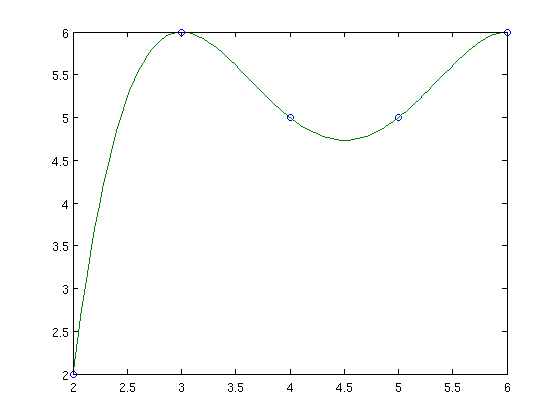
We, finally, plot the plynomial together with the points of \(C\).
xx=linspace(min(x),max(x));
yy=polyval(aa,xx);                   % polyval
                                     % Input: aa -> coefficients
                                     % xx -> vector of points where polynomial is evaluated
                                     % Output: yy -> values of polynomial
plot(x,y,'o',xx,yy)
The Matlab function to compute the Vandermonde's Matrix is vander. However, the order of columns is different than that of our construction.
vander(x)
ans =

          16           8           4           2           1
          81          27           9           3           1
         256          64          16           4           1
         625         125          25           5           1
        1296         216          36           6           1
In general, the matrix of Vandermonde is ill-conditioned, so this method is not used in practice but for theoretical analysis.
Lagrange interpolation
For each \(k=0,1,\ldots,n\), there exists a unique polynomial \(\ell_{k}\) of degree \(\leq n\) such that \(\ell_{k}\left(x_{j}\right)=\delta_{kj}\) (one if \(k=j\), zero otherwise): \[ \ell_{k}\left(z\right)= \frac{(z-x_{0})\ldots(z-x_{k-1})(z-x_{k+1})\ldots(z-x_{n})}{(x_{k}-x_{0}) \ldots(x_{k}-x_{k-1})(x_{k}-x_{k+1})\ldots(x_{k}-x_{n})}. \]
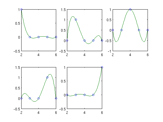
\(\ell_{0},\ell_{1},\ldots,\ell_{n}\) are the Lagrange fundamental polynomials. We shall create a function to compute the \(5\) Lagrange polynomials corresponding to the set of points \(C\). We'll do it in several steps:
Exercise 5.2. Write a function p=pro(x,z) to compute the product \[ (z-x_{0})(z-x_{1})\ldots(z-x_{n}) \] Use it with z=1.5.
p=pro(x,1.5)
p =

  -29.5312
Exercise 5.3. Modifying the function above, write another function p=produ(k,x,z) to perform the product \[ (z-x_{0})\ldots(z-x_{k-1})(z-x_{k+1})\ldots(z-x_{n}) \] Use it for k=3 and z=1.5.
p=produ(3,x,1.5)
p =

   11.8125
Exercise 5.4. Modifying the function above, write another function la=lagrange(k,x,z) to compute \[ \frac{(z-x_{0})\ldots(z-x_{k-1})(z-x_{k+1})\ldots(z-x_{n})}{(x_{k}-x_{0})\ldots(x_{k}-x_{k-1})(x_{k}-x_{k+1})\ldots(x_{k}-x_{n})} \] Use it for k=3 and z=1.5.
la=lagrange(3,x,1.5)
la =

    2.9531
Exercise 5.5 Transform function la=lagrange(k,x,z) to set z and la as vectors, i.e., to obtain as output the value of the Lagrange fundamental polynomial at several points. Use it for k=3 and z=[1.5 2.5 3.5].
la=lagrange(3,x,[1.5 2.5 3.5])
la =

    2.9531   -0.5469    0.7031
Now we make a plot of the polynomials
n=length(x);
y0=eye(n);    % Identity matrix n x n
              % Each row gives the value of Lagrange fundamental
              % polynomials for each node (blue circles)
for i=1:n
    subplot(2,3,i)
    yy=lagrange(i,x,xx);
    plot(x,y0(i,:),'o',xx,yy)
end
The Lagrange interpolation polynomial in the points \(x_{0,}x_{1},\ldots,x_{n}\) relative to the values \(y_{0},y_{1},\ldots,y_{n}\) is \[ P_{n}\left(x\right)=y_{0}\ell_{0}\left(x\right)+ y_{1}\ell_{1}\left(x\right)+\cdots+y_{n}\ell_{n}\left(x\right) \]
Let's compute and plot our solution for \(P_4\) \[ P_4(x)=y_{0}\ell_{0}(x)+\cdots+y_{4}\ell_{4}(x) \]
close all
n=length(x);
nn=length(xx);
yy=zeros(1,nn);
for i=1:n
    yy=yy+y(i)*lagrange(i,x,xx);
end
plot(x,y,'o',xx,yy)

The main drawback of this method is that, to add new data, we must recompute all the polynomials. To overcome this difficulty we use divided differences.
Lagrange interpolation. Divided differences
Newton's formula
We may write the Lagrange interpolating polynomial in \(x_{0,}x_{1},\ldots,x_{n}\) relative to \(y_{0},y_{1},\ldots,y_{n}\) as \[ P_{n}\left(x\right)= \left[y_{0}\right]+\left[y_{0},y_{1}\right]\left(x-x_{0}\right)+ \left[y_{0},y_{1},y_{2}\right]\left(x-x_{0}\right)\left(x-x_{1}\right)+\cdots +\left[y_{0},y_{1},\ldots,y_{n}\right]\left(x-x_{0}\right)\left(x-x_{1}\right)\cdots\left(x-x_{n-1}\right) \]
Table for divided differences
The coefficients of the Lagrange interpolating polynomial are computed in the following way: \[ \begin{array}{cccccc} x_{0} & y_{0} & \left[y_{0},y_{1}\right]=\frac{y_{0}-y_{1}}{x_{0}-x_{1}} & \left[y_{0},y_{1},y_{2}\right]=\frac{\left[y_{0},y_{1}\right]-\left[y_{1},y_{2}\right]}{x_{0}-x_{2}} & \ldots & \left[y_{0},y_{1},\ldots,y_{n}\right]=\frac{\left[y_{0},\ldots,y_{n-1}\right]-\left[y_{1},\ldots,y_{n}\right]}{x_{0}-x_{n}}\\ x_{1} & y_{1} & \left[y_{1},y_{2}\right]=\frac{y_{1}-y_{2}}{x_{1}-x_{2}} & \left[y_{1},y_{2},y_{3}\right]=\frac{\left[y_{1},y_{2}\right]-\left[y_{2},y_{3}\right]}{x_{1}-x_{3}} & \ldots\\ x_{2} & y_{2} & \left[y_{2},y_{3}\right]=\frac{y_{2}-y_{3}}{x_{2}-x_{3}} & \left[y_{2},y_{3},y_{4}\right]=\frac{\left[y_{2},y_{3}\right]-\left[y_{3},y_{4}\right]}{x_{2}-x_{4}} & \ldots\\ \ldots & \ldots & \ldots & \ldots & \ldots\\ x_{n-1} & y_{n-1} & \left[y_{n-1},y_{n}\right]=\frac{y_{n-1}-y_{n}}{x_{n-1}-x_{n}}\\ x_{n} & y_{n} \end{array} \]
Thus, if we add new data, we don't have to recompute all the differences but add new rows to the table.
Exercise 5.6. Write a function a=difdiv(x,y) to compute the matrix a containing the table of divided differences for the points in the vectors x and y. Don't store the first column, x, in a. Use matrix a to compute the interpolant in Newton's form. Plot the polynomial and the points.
x=[2,3,4,5,6];
y=[2,6,5,5,6];
a=difdiv(x,y)
a =

    2.0000    4.0000   -2.5000    1.0000   -0.2500
    6.0000   -1.0000    0.5000         0         0
    5.0000         0    0.5000         0         0
    5.0000    1.0000         0         0         0
    6.0000         0         0         0         0
[xx yy]=pol_newton(x,a);
plot(x,y,'o',xx,yy)

Matlab functions for interpolation
Interpolating polynomial. We use polyfit for defining and evaluating a polynomial.
pol=polyfit(x,y,length(x)-1); % output: polynomial coefficients
Plotting:
yy=polyval(pol,xx);
plot(x,y,'o',xx,yy)
close all
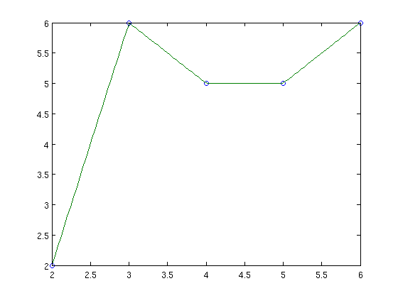
Piece-wise linear interpolation. We use function interp1:
yy=interp1(x,y,xx);
plot(x,y,'o',xx,yy)
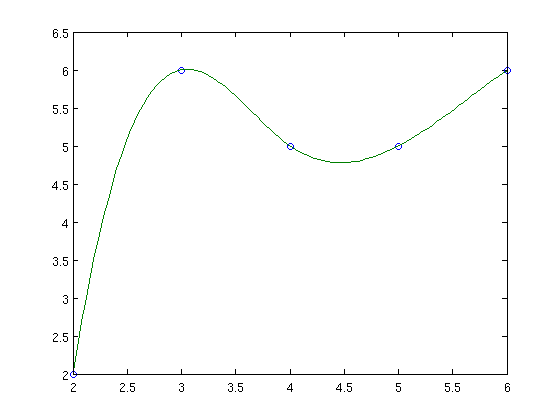
Spline interpolation. We use function spline:
yy = spline(x,y,xx);
plot(x,y,'o',xx,yy)
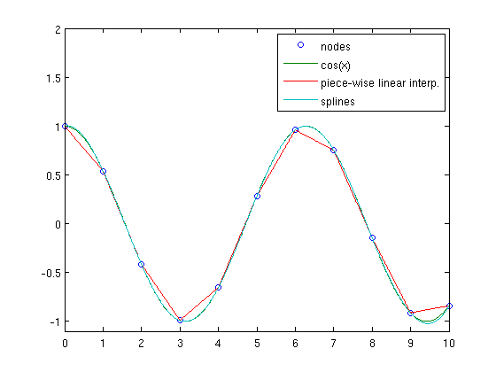
Exercise 5.7. Write a script, error_max.m, for interpolating function \(\cos x\) in the interval \([0,10]\) for the nodes \(x=0,1,\ldots,10\) and for plotting the resulting interpolants, in the cases:
- Piece-wise linear.
- Splines.
Then, compute for points=0:0.01:10 the maximum error point by point.
error_max
Error piece-wise linear = 0.12207
Error splines = 0.024833