Interpolation. Applications to image processing

Contents

Rigid transformations

One important application interpolation is the rigid transformation of images. Let \((i,j)\) denote the pixels of an image and \(I(i,j)\) their corresponding intensities. By rigid transformation we mean a linear transformation of the pixel coordinates, i.e. \[ \left(\begin{array}{cc}p\\q\end{array}\right)= A \left(\begin{array}{cc}i\\j\end{array}\right) \]

where \(A\) is a \(2\times 2\) matrix.

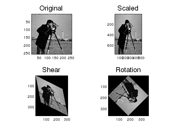
Among rigid transformations, we find the subclass of affine transformations. Here we use matlab for resizing, rotation and shear. To do this, we define a \(3\times 3\) matrix of the form \[ \left(\begin{array}{ccc}a_{11} & a_{12} & 0\\a_{21}& a_{22} & 0\\ 0 & 0 & 1\end{array}\right) \] and use the commands maketform and imtransform.

I=imread('cameraman.tif');
I=double(I);

s=[2,3];
tform1 = maketform('affine',[s(1) 0 0; 0 s(2) 0; 0 0 1]);       % scaling
I1 = imtransform(I,tform1);

sh=[0.5 0.2];
tform2 = maketform('affine',[1 sh(1) 0; sh(2) 1 0; 0 0 1]);     % shear
I2 = imtransform(I,tform2);

theta=3*pi/4;                                                   % rotation
A=[cos(theta) sin(theta) 0; -sin(theta) cos(theta) 0; 0 0 1];
tform3 = maketform('affine',A);
I3 = imtransform(I,tform3);

figure
subplot(2,2,1),imagesc(I),axis image
title('Original','FontSize',18)
subplot(2,2,2),imagesc(I1),axis image
title('Scaled','FontSize',18)
subplot(2,2,3),imagesc(I2),axis image
title('Shear','FontSize',18)
subplot(2,2,4),imagesc(I3),axis image
title('Rotation','FontSize',18)
colormap(gray)

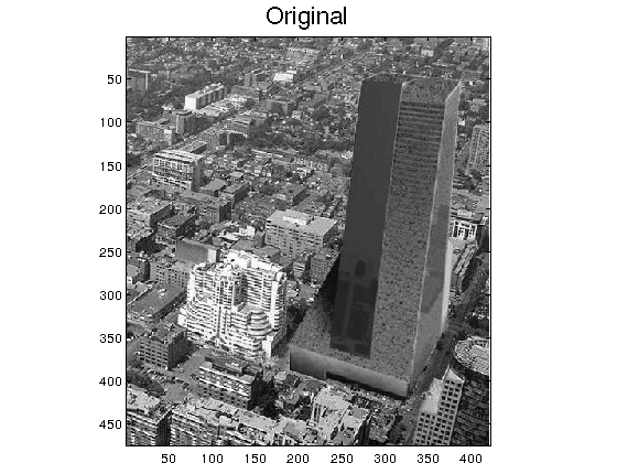
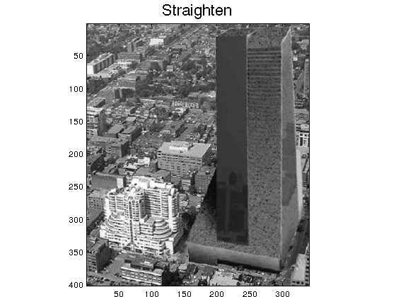
Exercise 5.1 We want to straighten the tower of the picture tower_bw.jpg. To do that we have to rotate it a suitable angle. But once we rotate it, a non-defined region appears (black in the figure). So then, we have to crop (manually) the image to eliminate that region. Make a script to perform this task. Show the initial and final images and the correction applied (in degrees).

Hint: Use a vertical line to decide if the tower is straight. For instance, if your rotated image is \(I\), then set \(I(:,9:12)=255\) to draw a vertical white line in columns 9 to 12.

%The result is:

Exercise5_1

correction (degrees) -> -7.2

Nonlinear transformations

This is the case when, in the transformation \[ \left(\begin{array}{cc}p\\q\end{array}\right)= A \left(\begin{array}{cc}i\\j\end{array}\right) \] the matrix \(A\) may depend on the particular pixel in which it is acting, i.e. in \((i,j)\), in the above notation.

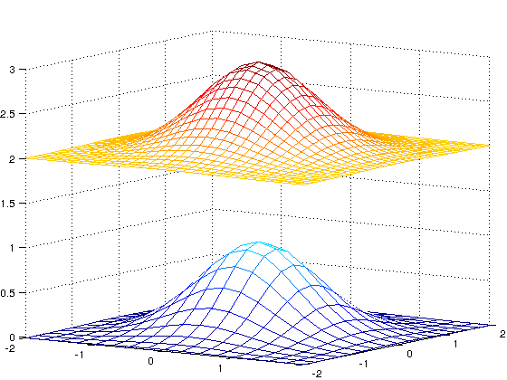
For these transformations, we use the Matlab command interp2, which interpolates functions defined in a 2D domain. For instance, we consider \(f(x,y)=e^{-x^2-y^2}\) given in a coarser grid and then compute its values in a finer grid. The plots are

clear
[x,y] = meshgrid(-2:0.25:2);            % coarser grid
z = exp(-x.^2-y.^2);
[p,q] = meshgrid(-2:0.125:2);           % finer grid
zfinal = interp2(x,y,z,p,q);            % interpolation
mesh(x,y,z), hold on
mesh(p,q,zfinal+2)
colormap(jet)
view([34,10])

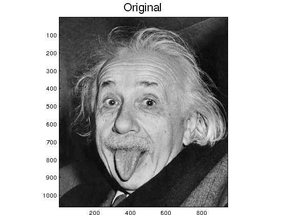
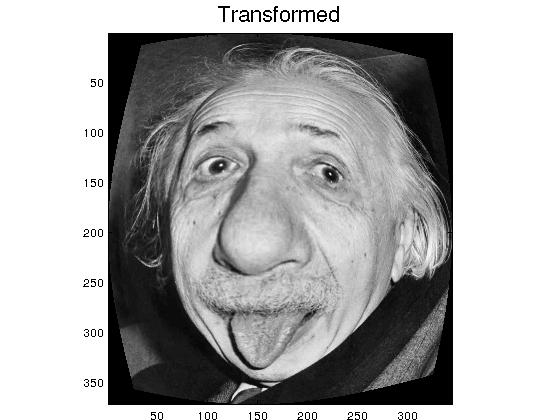
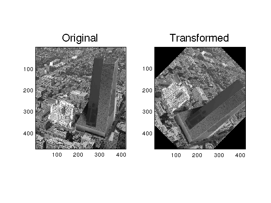
Command interp2 may be used for affine transformations too. For instance, we rotate \(\theta\) radians the tower image with center at \((x_0,y_0)\): \[ \left(\begin{array}{c}p \\ q\end{array}\right)= \left(\begin{array}{cc}\cos(\theta) & \mathrm{sen}(\theta)\\ -\mathrm{sen}(\theta)& \cos(\theta) \end{array}\right) \left(\begin{array}{c}x-x_0 \\ y-y_0\end{array}\right) +\left(\begin{array}{c}x_0 \\ y_0\end{array}\right) \]

clear all
I=imread('tower_bw.jpg');
I=im2double(I);
m=size(I,1);n=size(I,2);
[x,y] = meshgrid(1:n,1:m);                    % grid inherited from the original image

theta=pi/4;                                   % angle of rotation
x0=fix(n/2);y0=fix(m/2);                      % center of rotation
p=(x-x0).*cos(theta)+(y-y0).*sin(theta)+x0;   % transformed coordinates (new pixel locations)
q=-(x-x0).*sin(theta)+(y-y0).*cos(theta)+y0;

Ifinal=interp2(x,y,I,p,q,'bicubic');          % intensity values interpolation at new locations

figure
subplot(1,2,1),imagesc(I),axis image
title('Original','FontSize',18)
subplot(1,2,2),imagesc(Ifinal),axis image
title('Transformed','FontSize',18)
colormap(gray)

Exercise5_2 The goal of this exercise is to introduce an eddy in the swimingpool, as shown in the figure (final result of the exercise)

Exercise5_2

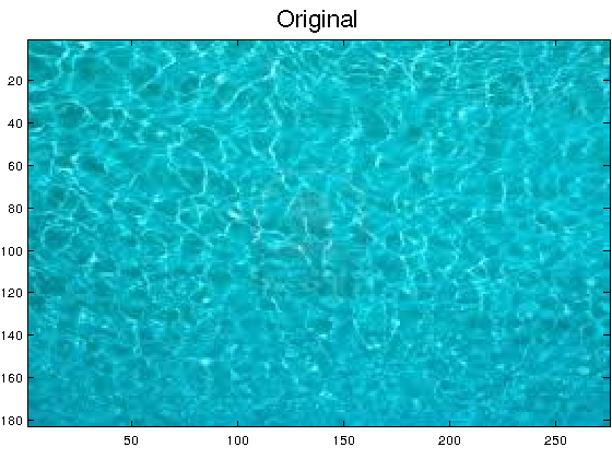
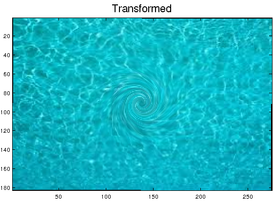
To complete this exercise, use the rotation script above, introducing the following changes:

If the picture were a intensity image, then we would just use interp2 as above. Since our picture is a rgb image, we have to use the interpolation for each color channel. To do this, we use a loop in this way

% Ifinal=zeros(size(Ic));               % initialize the final matrix
% for k=1:3 % colors
    % select first channel
    % interpolate and produce Ichannel;
    % Ifinal(:,:,k)= Ichannel;          % add k channel
% end
% Ifinal=im2uint8(Ifinal);              % convert to unsigned integer

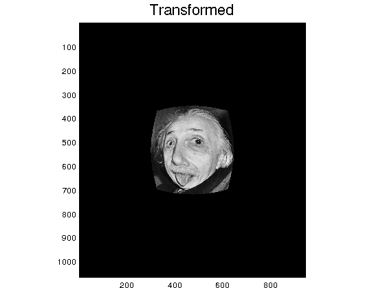
Exercise5_3 The goal of this exercise is to introduce a non uniform scaling of an image. We also want to introduce automatic cropping.

In this case, we define the transformation as \[ \begin{array}{ll}p=d*r(x,y).*(x-x0)+x\\ q=d*r(x,y).*(y-y0)+y, \end{array}\] for \(d=0.01\). After interpolation, we get a small picture full of non-defined intensity values. But the final result should be

Exercise5_3

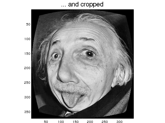
By using the function find, locate the pixels at which the interpolated image is positive. Then, define another image restricted to this set of indices.

Exercise 5_4 Modify the script of Exercise5_3 to make a function with

Use it. For instance

I=imread('einstein_bw.jpg');
A=Exercise5_4(I,361,593,0.01);

Published with MATLAB® 7.14