Fourier approximation. Applications to Image Processing

Contents

2D Fourier transform

Let \(f(x,y)\) denote an \(M\times N\) image, for \(x=0,1,2,\ldots,M-1\) and \(y=0,1,2,\ldots,N-1\). The 2D discrete Fourier Transform (DFT) of \(f\), denoted by \(F(m,n) \), is given by \[ F(m,n)= \sum_{x=0}^{M-1}\sum_{y=0}^{N-1} f(x,y) \exp(-2\pi i(\frac{x}{M}m+\frac{y}{N}n)).\] for \(m=0,1,2,\ldots,M-1\) and \(n=0,1,2,\ldots,N-1\). The \(M\times N\) rectangular region defined for \( (m,n)\) is called the frequency domain, and the values of \(F(m,n)\) are called the Fourier coefficients.

The inverse discrete Fourier transform is given by \[ f(x,y)=\frac{1}{MN}\sum_{m=0}^{M-1}\sum_{n=0}^{N-1} F(m,n) \exp(2\pi i(\frac{m}{M}x+\frac{n}{N}y)),\] for \(x=0,1,2,\ldots,M-1\) and \(y=0,1,2,\ldots,N-1\).

Remark. In some formulations of the DFT the \(1/MN\) term is placed in front of the transform and in others it is used in front of the inverse. Still, in others, a term \(1/\sqrt{MN}\) is placed in both. We have placed it in front of the inverse to be consistent with Matlab. Also, observe that indices, in Matlab, start with \(1\) rather than \(0\).

Even if \(f(x,y)\) is real, its transform \(F(m,n)\) is in general a complex function. For visualization, we use the power spectrum, \(P(m,n)= F(m,n) \bar F(m,n)\), where \(\bar F\) denotes the complex conjugate of \(F\).

Two properties.

The DFT and its inverse are obtained in practice using a fast Fourier Transform. In Matlab, this is done using the command fft2: F=fft2(f). To compute the power spectrum, we use the Matlab function abs: P=abs(F)^2. If we want to move the origing of the transform to the center of the frequency rectangle, we use Fc=fftshift(F). Finally, if we want to enhance the result, we use a \(log\) scale.

Examples

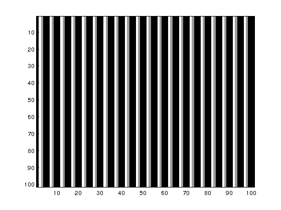
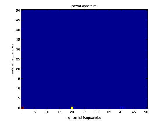
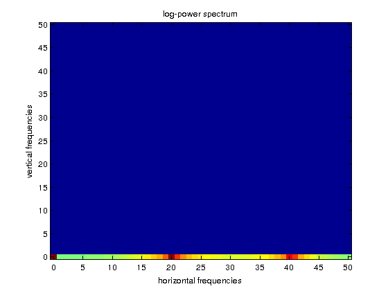
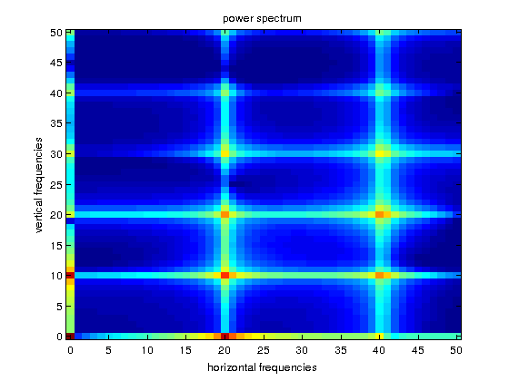
Example 6.3. We load an image periodic in the horizontal direction. In the first figure we see the image. The second figure corresponds to the power spectrum, P, of the image, for which a maximum at \((0,20)\) is visualized as a yellow rectangle. In the third figure, we plot \(\log(1+P)\) to enhance the visualization. We see that \((0,40)\) is also a relative maximum for the power spectrum. This maximum corresponds to what is called the first harmonic \( (2*20)\) of the fundamental frequency \((20)\). Finally, observe that, like in the 1D case, by symmetry considerations, we only need to plot half of the horizontal and vertical frequency ranges.

f=imread('lines.tif'); % integer type
f=double(f); % to make computations in double precission
[M,N]=size(f);
figure,imagesc(f),colormap(gray)
F=fft2(f)/sqrt(M*N); % observe the normalization
cF=fftshift(F); % centering in the origin
cP=abs(cF).^2;
Mrange=0:floor(M/2); % ranges for the representation
Nrange=0:floor(N/2);
figure,imagesc(Mrange,Nrange,cP(floor(M/2)+1:M,floor(N/2)+1:N)), axis xy,
title('power spectrum'), xlabel('horizontal frequencies'), ylabel('vertical frequencies')
figure,imagesc(Mrange,Nrange,log(1+cP(floor(M/2)+1:M,floor(N/2)+1:N))), axis xy,
title('log-power spectrum'), xlabel('horizontal frequencies'), ylabel('vertical frequencies')

Notice that we divided by \(\sqrt{MN}\) to normalize the energy. In this way \(\left\|f\right\|=\left\|fF\right\|\):

out1=norm(F);
out2=norm(double(f)); % norm is not defined for uint8
fprintf('out1=%d out2= %d\n',out1,out2)

out1=1.283468e+04 out2= 1.283468e+04

The normalization for the inverse Fourier transform (ifft2) is got by multiplying by \(\sqrt{MN}\)

f2=ifft2(F)*sqrt(M*N);
f2=real(f2);% chopping small complex values due to rounding errors
out3=norm(f2);
fprintf('out3=%d ',out3)

out3=1.283468e+04 

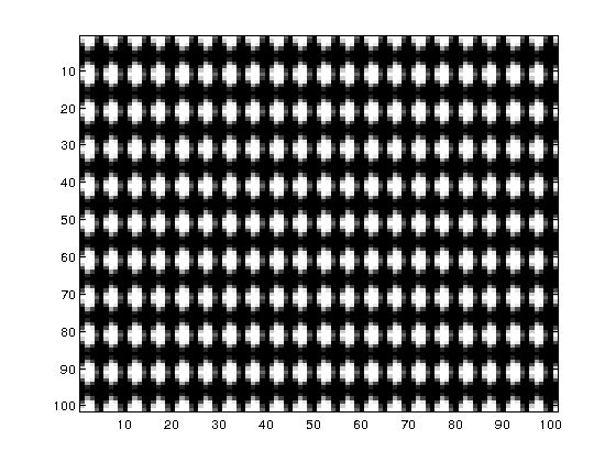
Example 6.4. Now we load an image perodic in both directions and plot the image and the \(\log(1+P)\). In this case, the maximum corresponds to the frequencies \((20,10)\). The corresponding harmonics are also visible as local maxima.

f=imread('dots.tif'); % integer type
f=double(f); % to make computations in double precission
[M,N]=size(f);
figure,imagesc(f),colormap(gray)
F=fft2(f)/sqrt(M*N); % observe the normalization
cF=fftshift(F); % centering in the origin
cP=abs(cF).^2;
Mrange=0:floor(M/2); % ranges for the representation
Nrange=0:floor(N/2);
figure,imagesc(Mrange,Nrange,log(1+cP(floor(M/2)+1:M,floor(N/2)+1:N))), axis xy
title('power spectrum'), xlabel('horizontal frequencies'), ylabel('vertical frequencies')

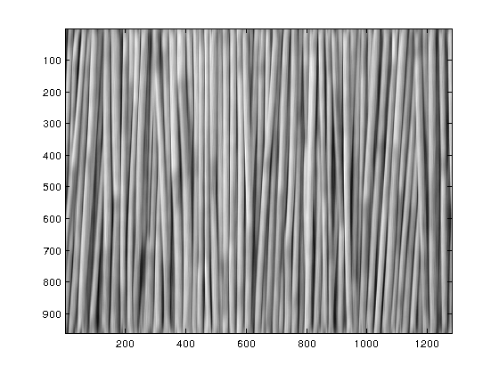
Example 6.5. We finally test a natural image which has a strong horizontal frequency component, as it is showed by the alignment of relative maxima in the horizontal axis of \(\log(1+P)\). In this case, we have plotted the whole frequency ranges, for a better visualization of the horizontal \(X=0\) axis. Notice the symmetry with respect to both axis.

f=imread('canes.jpg');
f=rgb2gray(f);
f=double(f);
[M,N]=size(f);
figure,imagesc(f),colormap(gray)
F=fft2(f)/sqrt(M*N);
cF=fftshift(F); % centering in the origin
cP=abs(cF).^2;
figure,imagesc(-floor(M/2):floor(M/2),-floor(N/2):floor(N/2),log(1+cP)), axis xy % we plot the whole range
title('power spectrum'), xlabel('horizontal frequencies'), ylabel('vertical frequencies')

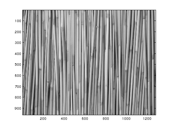
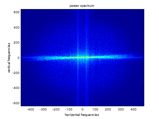
Image thresholding

An image is recovered from the set of coefficients \(F\) by using the inverse Fourier Transform (Matlab function ifft2). As we have seen, in general, not all the coefficients have the same value. In order to use only the most important, we may select those that are larger in modulus than some given threshold \(T\), i.e. we set to zero all the coefficients but those contained in the following set: \[ S_T=\left\{0\leq m\leq M-1, 0\leq n \leq N-1 : \left| F(m,n)\right| \geq T\right\} .\]

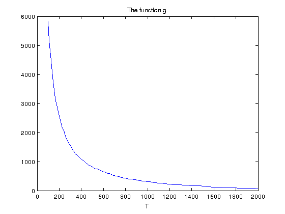
Let us denote by \(g(T)\) the number of indices in \(S_T\). One one hand, for \(T=0\) we have \(g(0)= MN\), since \(\left| F(m,n)\right| \) is always non-negative. On the other hand, for \(T> \max \left| F(m,n)\right| \) we obviously have \(g(T)=0\). Observe that \(g\) is a decreasing function of \(T\). We construct here a plot of \(g\) using the command nnz, which gives the number of non zero elements of a matrix.

g=[];
aF=abs(F);
for T=100:10:2000
    g=[g nnz(aF >=T)];
end
plot(100:10:2000,g), title('The function g'), xlabel('T')

Now we perform a thresholding, i.e., set to zero all the coefficients which are smaller than a fixed \(T\). How do we choose \(T\)? To start with,

We take, for instance \(T=100\) and look at the result:

T=100;
c=F.*(abs(F)>=T);
fM=real(ifft2(c))*sqrt(M*N);
imagesc(fM),colormap(gray)

We, finally, compute the ratio between the number of nonzero coefficients of the Fourier transform, \(F\), and that of the thresholded matrix \(c\):

out1=nnz(F);   % for recovering the exact image
out2=nnz(c);    % for the thresholded image
out3=out1/out2; % compression ratio
fprintf('out1=%d out2=%d out3=%d\n',out1,out2,out3)

out1=1228800 out2=5823 out3=2.110252e+02

Exercise

For a given image of size \(M\times N\), we want to compress it at some given ratio \(r\) by keeping the most significative Fourier coefficients, i.e., we want to determine the threshold, \(T\), such that the compression ratio equals \(r\). In other words, we want to compute \(T\) such that \( \frac{g(T)}{MN}=r \). To do this, we compute the zero of the function \[h(T)=g(T) -rMN.\] Follow these steps to write the script compression.m:

Published with MATLAB® 7.14