Numerical differentiation

First derivative of a one-variable function
Second derivative of one-variable function
Differentials of two-variable functions

First derivative of a one-variable function

We seek for approximating $f'$ in $\hat x \in [a,b]\subset \mathbb{R}$ by using $f$-values in a small number of points close to $\hat x$.

The two main reasons to do this are:

Funtion $f$ is known only at some finite number of points.
It's cheaper computing the approximation than the exact value.

From the definition of derivative \[ f'(\hat x)=\lim_{h\to0}\frac{f(\hat x+h)-f(\hat x)}{h} \]

we obtain three main approximation finite differences schemes: \[ \textbf{Forward: } (\delta^+ f)( x_{i})=\frac{f(x_{i+1})-f( x_{i})}{h}, \qquad\textbf{Backward: } (\delta^- f)( x_{i})=\frac{f(x_{i})-f(x_{i-1})}{h}, \qquad\textbf{Centered: }(\delta f)(x_{i})=\frac{1}{2}\big((\delta^+ f)(x_{i})+(\delta^- f)(x_{i})\big)= \frac{f(x_{i+1})-f(x_{i-1})}{2h} \]

Observe that with these formulas we can not compute the derivative at, at least, one of the extremes of the interval. For instance, $(\delta^+ f)(b)$ needs the value $f(b+h)$ which, in general, is unknown.

Matlab commands. Matlab is more efficient when vectorizing computations. For the exercises below, you may find useful the command diff(X), which computes $(X_2-X_1, X_3-X_2,\ldots,X_n-X_{n-1})$, and the command norm(X) which computes the Euclidean norm of vector $X$, i.e. \[ \text{norm}(X)=\sqrt{\sum_{i=1}^n X_i^2}.\]

Exercise 7.1. For the function $f(x)=e^x$ in $[0,1]$, and for $h=0.1$ and $h=0.01$:

Compute and plot the exact derivative in the interval $[h,1-h]$.
Compute and draw, in the same plot than above and in the same interval, the approximate derivatives $df_f$, $df_b$ and $df_c$ by using forward, backward and centered schemes, respectively.
Compute and draw, in a new figure, the pointwise erros $f'(x_i)-df_a(x_i)$, where $x_i$ are the points of the mesh and $a=f,~b$ or $c$.
Compute the global relative error of each approximation \[ \text{norm}(X)=\sqrt{\frac{\sum_{i=1}^n (f'(x_i)-df_a(x_i))^2}{\sum_{i=1}^n (f'(x_i))^2}}.\]

The solution is:

Exercise7_1

step size and global relative errors (h,f,b,c) = 	0.010	 5.016708e-03	 4.983375e-03	 1.666675e-05
step size and global relative errors (h,f,b,c) = 	0.001	 5.001667e-04	 4.998334e-04	 1.666667e-07

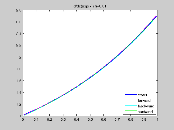
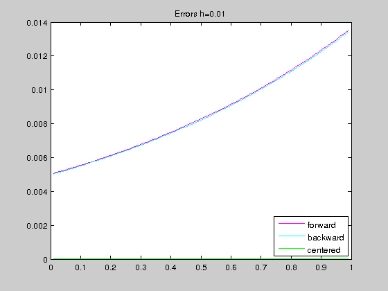
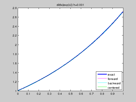
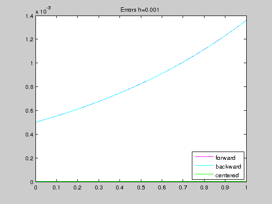
We see that the centered scheme gives better results. This is because forward and backward schemes are of order 1 while centered scheme is of order 2.

As mentioned above, on the extremes of the interval, all the schemes need to evaluate $f$ outside the interval $[a,b]$. To override this difficulty we shall use the 2nd order Lagrange interpolating polynomial for $x_1$, $x_2$, $x_3$, being $y_j=f(x_j)$. We have

\[ p(x)=[y_1]+[y_1,y_2](x-x_1)+[y_1,y_2,y_3](x-x_1)(x-x_2),\]

with \[[y_1]=y_1,\quad [y_1,y_2]=\frac{y_1-y_2}{x_1-x_2}=\frac{y_2-y_1}{h}, \quad [y_1,y_2,y_3]=\frac{[y_1,y_2]-[y_2,y_3]}{x_1-x_3}=\frac{1}{2h}(\frac{y_1-y_2}{h} -\frac{y_2-y_3}{h}\big)= \frac{1}{2h^2}(y_1-2y_2+y_3),\]

and therefore, we deduce \[ f'(x_1)\approx p'(x_1)=\frac{1}{2h}(-3f(x_1)+4f(x_2)-f(x_3)), \qquad f'(x_3)\approx p'(x_3)=\frac{1}{2h}(f(x_1)-4f(x_2)+3f(x_3)) \qquad (1)\]

Exercise 7.2. For $f(x)=\frac{1}{x}$ in $[0.2,1.2]$, and $h=0.01$:

Compute the approximate derivative in the interval $[0.2,1.2]$ by using a centered scheme in the interior points and forward and backward schemes on $x=0.2$ and $x=1.2$, respectively.
Compute the approximate derivative by using a centered scheme in the interior points and the formulas deduced in (1) on $x=0$ and $x=1$, respectively.
Compute the exact derivative in the interval $[0.2,1.2]$, and then the global relative error of each approximation.

The solution is:

Exercise7_2

step size and global relative errors (h,order 1,order 2) = 	0.01	 1.786397e-02	 2.171714e-03

Second derivative of one-variable function

From the interpolating polynomial \[ p(x)=[y_1]+[y_1,y_2](x-x_1)+[y_1,y_2,y_3](x-x_1)(x-x_2) \] we obtain \[p''(x_2)=2[y_1,y_2,y_3]= \frac{1}{h^2}(y_1-2y_2+y_3)\qquad (2)\]

Exercise 7.3. For $f(x)=\sin(2\pi x)$ in $[0,1]$, and $h=0.01$:

Compute the exact second derivative, the approximate second derivative according to formula (2), and the relative error of the approximation in the interval $[h,1-h]$. You may want to use the Matlab command diff(X,2).

The solution is:

Exercise7_3

step size and global relative error (h, RE) = 	0.01	 3.289435e-04

Differentials of two-variable functions

Lat $\Omega = [a,b]\times[c,d]\subset \mathbb{R}^2$ and consider uniform partitions \begin{eqnarray*} a=x_1<x_2<\ldots<x_{M-1}<x_M=b \\ c=y_1<y_2<\ldots<y_{N-1}<y_N=d \end{eqnarray*} Denote a point of $\Omega$ by $(x_m,y_n)$. Then, its neighbor points are

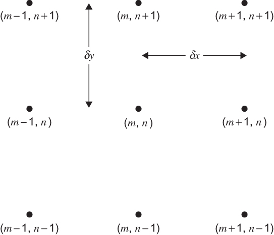
We may use the same ideas than those used for scalar functions. For instance

x-partial derivative (forward): $\partial_x f(x_m,y_n)$ \[ (\delta_x^+f)(x_m,y_n)= \frac{f(x_{m+1},y_n)-f(x_{m},y_n)}{h_x} \]

Gradient (centered): $\nabla f(x_m,y_n)=(\partial_x f(x_m,y_n),\partial_y f(x_m,y_n))$ \[ (\frac{f(x_{m+1},y_n)-f(x_{m-1},y_n)}{2h_x}, \frac{f(x_{m},y_{n+1})-f(x_{m},y_{n-1})}{2h_y})\quad (2)\]

Divergence (centered): $\mathrm{div} \overrightarrow{f}(x_m,y_n)=\partial_x f_1(x_m,y_n)+\partial_y f_2(x_m,y_n)$ \[ \frac{f_1(x_{m+1},y_n)-f_1(x_{m-1},y_n)}{2h_x}+ \frac{f_2(x_{m},y_{n+1})-f_2(x_{m},y_{n-1})}{2h_y} \quad (3) \]
Laplacian (centered): $\Delta f(x_m,y_n)=\partial_{xx} f(x_m,y_n)+ \partial_{yy} f(x_m,y_n)$ \[ \frac{f(x_{m+1},y_n)-2f(x_m,y_n)+f(x_{m-1},y_n)}{h_x^2}+ \frac{f(x_{m},y_{n+1})-2f(x_m,y_n)+f(x_{m},y_{n-1})}{h_y^2} \quad (4) \]

Before entering into matter, let us recall the basics on plotting surfaces and vector functions with Matlab.

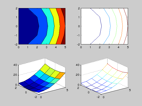
If we want to plot the escalar function $f(x,y)=x^2+y^2$ in $x \in [0,5]$ with step $h_x=1$ and $y \in [-2,2]$ with step $h_y=1$, we use

[x,y]=meshgrid(0:1:5,-2:1:2)

x =
     0     1     2     3     4     5
     0     1     2     3     4     5
     0     1     2     3     4     5
     0     1     2     3     4     5
     0     1     2     3     4     5
y =
    -2    -2    -2    -2    -2    -2
    -1    -1    -1    -1    -1    -1
     0     0     0     0     0     0
     1     1     1     1     1     1
     2     2     2     2     2     2

In this way we have generated two matrices with the components of the coordinates of the given domain. Now, we may compute the values of $z=f(x,y)=x^2+y^2$ for each pair $(x_{ij},y_{ij}) \quad i=1,\ldots,m,\,j=1,\ldots,n$, being $m$ and $n$ the number of rows and columns of $x$ and $y$ (their size, in Matlab notation).

f=@(x,y) x.^2+y.^2;
z=f(x,y)

z =
     4     5     8    13    20    29
     1     2     5    10    17    26
     0     1     4     9    16    25
     1     2     5    10    17    26
     4     5     8    13    20    29

With these matrices we have all what we need to plot $f$. Functions contour and surf are the most commonly used:

figure
subplot(2,2,1), contourf(x,y,z)
subplot(2,2,2), contour(x,y,z)
subplot(2,2,3), surf(x,y,z)
subplot(2,2,4), mesh(x,y,z)

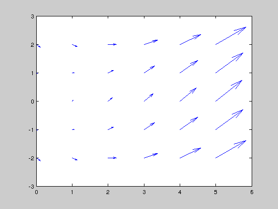
For plotting a vector function we use meshgrid and quiver:

u1=x.^2+y.^2;
u2=x.^2-y.^2;
figure, quiver(x,y,u1,u2)

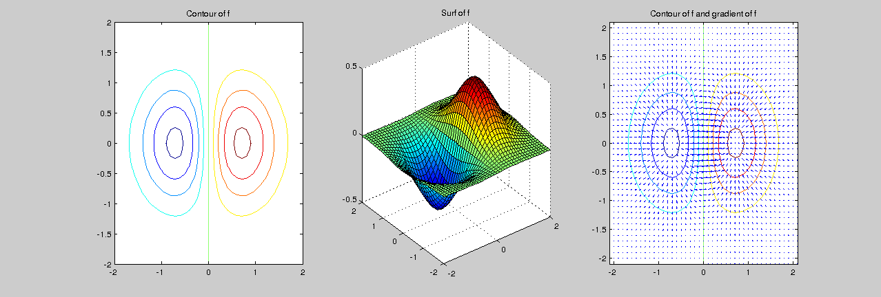
Exercise 7.4. In this exercise we compute the gradient of a function using Matlab command gradient: [fx,fy] = gradient(f,hx,hy), returns the numerical gradient of the matrix f, using the spacing specified by hx and hy.

Plot, using contour and surf, the function $f(x,y)=x e^{-x^2-y^2}$ in $[-2,2]\times[-2,2]$ with $h_x=h_y=0.1$.
Compute, using the Matlab function gradient, the gradient of $f$ and plot it together with a contour plot of $f$.
Compute the global relative error of the approximation using norm.

Exercise7_4

relative error = 	1.225674e-02

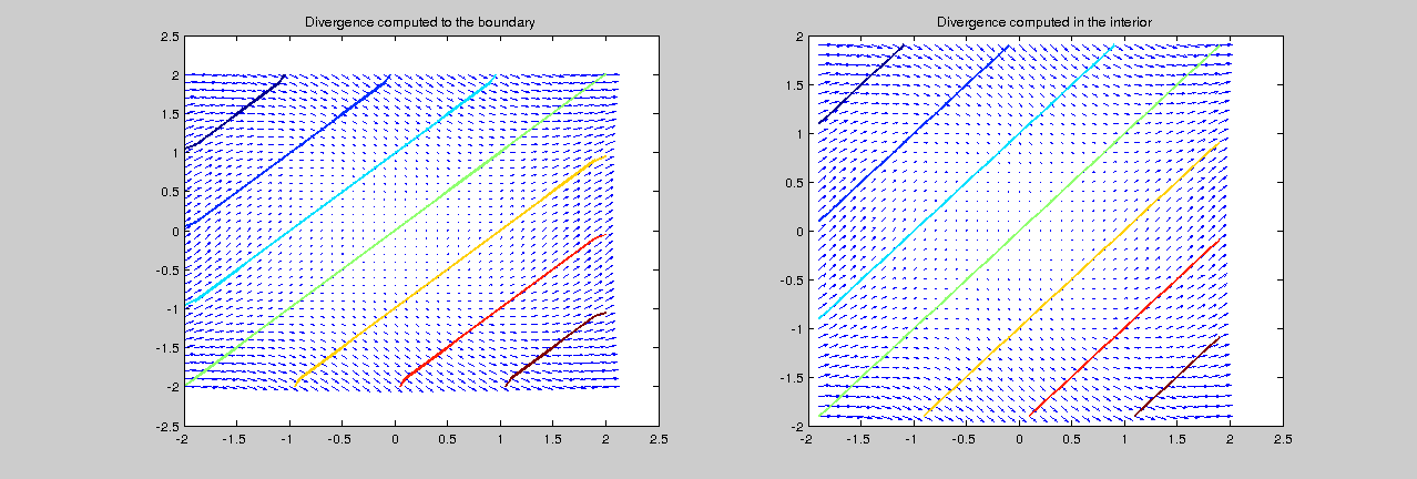
Exercise 7.5. In this exercise we compute the divergence of a vector function using Matlab command divergence: div = divergence(x,y,f1,f2) computes the divergence of a 2-D vector field $\mathbb{f}=(f_1(x,y),f_2(x,y))$. The arrays $x,y$ define the coordinates for $(f_1,f_2)$ and may be produced by meshgrid.

Compute, using Matlab command divergence, the divergence of $\mathbb{f}(x,y)=(x^2+y^2,x^2-y^2)$ in $[-2,2]\times[-2,2]$ with $h_x=h_y=0.2$. Then plot both $\mathbb{f}$ (using quiver) and $\text{div} (\mathbb{f})$ (using contour).
A boundary effect may be noticed in these plots due to the bad approximation of the divergence on these points. Remake the plots above restricting the set to $[-2+h_x,2-h_x]\times[-2+h_y,2-h_y]$
Compute the global relative errors of the approximation in both sets using norm.

Exercise7_5

relative error = 	9.333167e-03 2.698803e-16

Exercise 7.6. In this exercise we compute the laplacian of a function using Matlab command del2: $L = del2(f,h_x,h_y)$, when $f$ is a matrix, is a discrete approximation of $\frac{1}{4} (\partial_{xx} f(x,y)+\partial_{yy} f(x,y))$. The matrix $L$ is the same size as $f$, with each element equal to the difference between an element of $f$ and the average of its four neighbors.

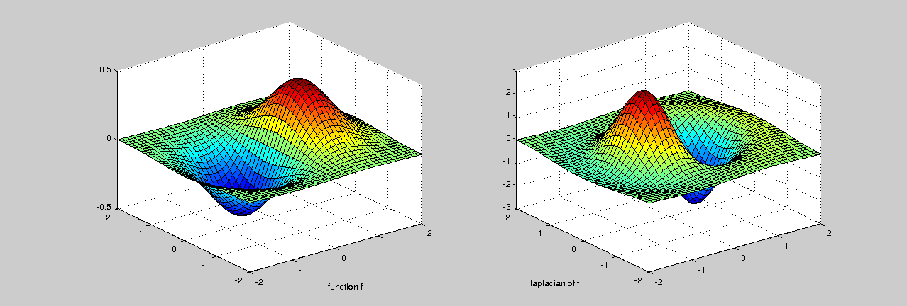
Compute, using Matlab command del2, the laplacian of $f(x,y)=x e^{-x^2-y^2}$ in $[-2,2]\times[-2,2]$ with $h_x=h_y=0.2$. Plot the function and its laplacian using surf.
Compute the exact solution and then the global relative error of the approximation using norm.

Exercise7_6

relative error = 	5.914553e-03

Numerical differentiation

Contents

First derivative of a one-variable function

Second derivative of one-variable function

Differentials of two-variable functions