Convolution
Contents
Convolution is an important application of integration. It is an operation in which:
- For a fixed kernel \(g:\mathbb{R}^n\to\mathbb{R}\), and
- For any input function \(f:\mathbb{R}^n\to\mathbb{R}\)
- The operation gives an output function, denoted as \(f*g:\mathbb{R}^n\to\mathbb{R}\), according to the formula \[f*g(x)=\int_{\mathbb{R}^n} g(x-y)f(y) dy.\]
The corresponding discrete version uses numerical integration. In the simplest one-dimensional situation we obtain \[f*g(x_i)=h \sum_{j=-\infty}^\infty g(x_i-x_j)f(x_j) \] where \(\{x_j\}\) is a uniform mesh of \(\mathbb{R}\) with step-size \(h\).
The border issue
When the convolution is taken in a bounded interval, the border issue arises. That is, for some \(x's\) near the border of the interval the product \(g(x_i-x_j)f(x_j)\) is not defined, since \(x_j\) may go beyond the border. There are several strategies to correct this situation. Next, we show an example in connection to the use of convolution for numerical differentiation.
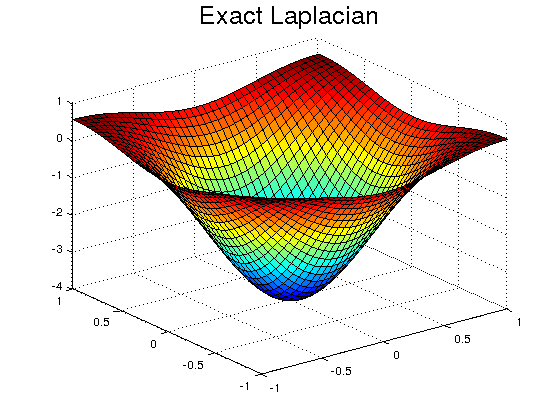
We start defining the function, its exact Laplacian and the Laplace convolution kernel in the square \( [-1,1]\times [-1,1]\).
f=@(x,y) exp(-(x.^2+y.^2));
Lf=@(x,y) 4*f(x,y).*(x.^2+y.^2-1); % exact Laplacian of f

h=0.05;% step of the mesh (for x and y axis)
[x,y]=meshgrid(-1:h:1);
[s1,s2]=size(x);

F=f(x,y);
Le=Lf(x,y); % exact discrete Laplacian

K=(1/h^2)*[0 1 0; 1 -4 1; 0 1 0]; % kernel to compute the Laplacian
figure
surf(x,y,Le)
title('Exact Laplacian','FontSize',20)
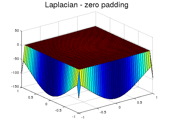
The first method is the zero-padding, i.e. extending \(f\) by zero outside its domain. We use the Matlab command conv2 to compute the two-dimensional convolution of two vectors.
FA=[zeros(1,s2+2);
    zeros(s1,1) F zeros(s1,1);
    zeros(1,s2+2)];
Lz=conv2(FA,K,'valid');% this option gives the result in the region without padding
figure
surf(x,y,Lz)
title('Laplacian - zero padding','FontSize',20)
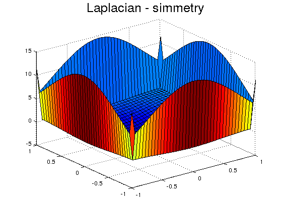
Another possibility is to extend the function by simmetry
FA=[0 F(1,:) 0;
    F(:,1) F F(:,end);
    0 F(end,:) 0];
Ls=conv2(FA,K,'valid');
figure
surf(x,y,Ls)
title('Laplacian - simmetry','FontSize',20)
Since in this example we know the exact function, we make the extension by extrapolation. In general this can not be done, since we don't know the values of the function outside its domain. Extrapolation must be done by other means.
[x1,y1]=meshgrid(-1-h:h:1+h);
FA=f(x1,y1);
Lx=conv2(FA,K,'valid');
figure
surf(x,y,Lx)
title('Laplacian - fake extrapolation','FontSize',20)
fprintf('Relative error-> %d',norm(Lx-Le)/norm(Le));
Relative error-> 1.016412e-03

The relative error order is the same as the step-size of the mesh.
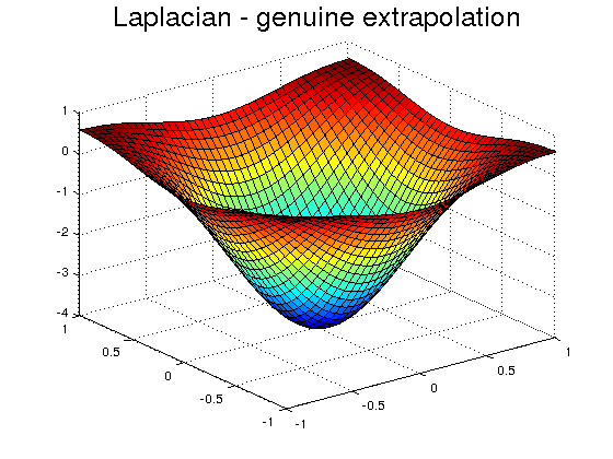
Finally, we use the Matab command del2 to compute the Laplacian. This command has implemented a extrapolation rule using only the values inside the domain, as it should.
Lm=4*del2(F,h);
figure
surf(x,y,Lm)
title('Laplacian - genuine extrapolation','FontSize',20)
fprintf('Relative error-> %d',norm(Lm-Le)/norm(Le));
Relative error-> 2.425621e-03
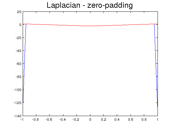
Exercise 1 We shall correct the border issue using a 2nd order approximation of the derivative at the border. Define the one-dimensional function \(f(x)=\exp(-x^2)\) and its Laplacian (second order derivative, computed by hand). Introduce the corresponding convolution kernel \(K=(1/h^2)*[1,-2,1]\), and the domain \( [-1,1]\) discretized with a uniform mesh of step-size \(h=0.01\). Then
- Produce the convolution zero-padding approximation of the Laplacian and plot it together with the exact Laplacian. Observe the border issue.
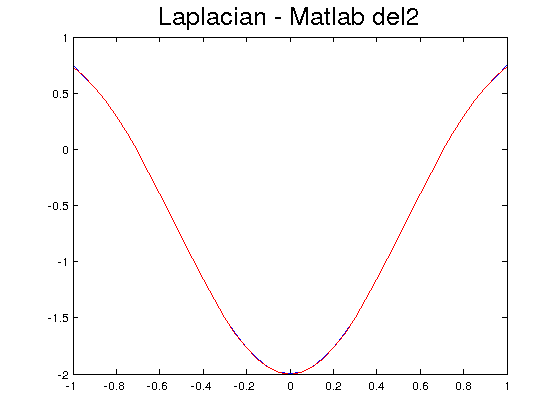
- Use the command del2 to produce the Laplacian approximation. Plot it together with the exact Laplacian and compute the relative error.
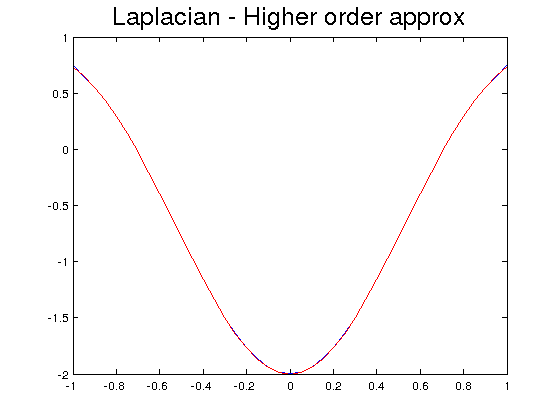
- Modify the zero-padding approximation of the Laplacian by replacing the first and last elements by the second order approximations given by \[ f''(x_1)=\frac{1}{h^2} (2f(x_1)-5f(x_2)+4f(x_3)-f(x_4))\] and the analogous formula for \(f''(x_{end})\). Then, plot it together with the exact Laplacian and compute the relative error.
The solution is
Exercise1
Relative error higher order -> 3.429893e-03
Relative error del2 -> 3.429893e-03
2D Convolution. Image filtering
There exist many image processing tasks performed in terms of convolution with an appropriate kernel.
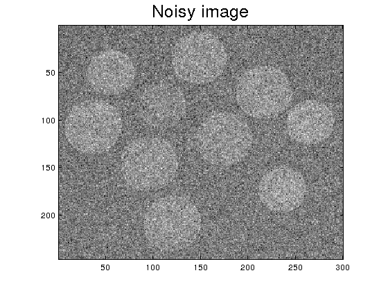
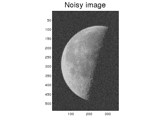
Step 1. We start reading the image and adding Gaussian noise
I0=imread('moon.tif');I0=im2double(I0);
noise=0.1;
I=I0+noise*randn(size(I0));
figure
imagesc(I),axis image,colormap('gray')
title('Noisy image','FontSize',20)
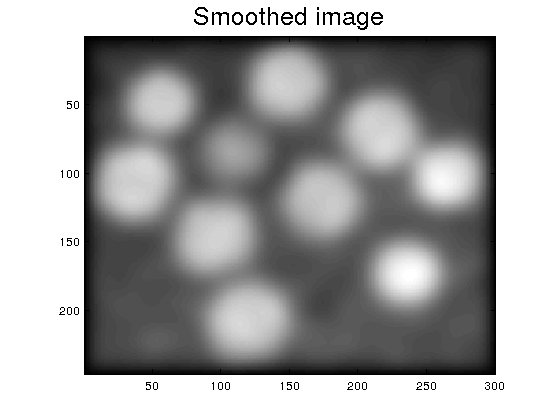
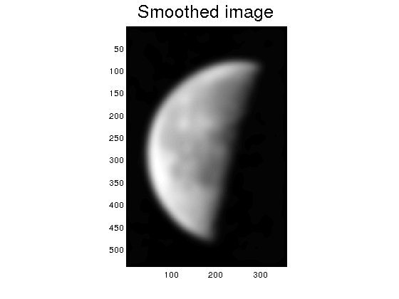
Step 2. We perform the iterated convolution with a smoothing kernel.
n=3;
kS=ones(n,n)/n^2; % smoothing kernel of order n
I1=I;
for k=1:100
    I2=conv2(I1,kS,'same');
    I1=I2;
end
figure
imagesc(I2),axis image,colormap('gray')
title('Smoothed image','FontSize',20)
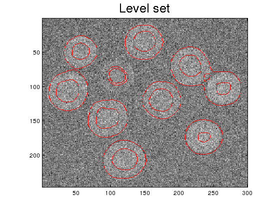
Step 3. We use the zero-crossing of the Laplacian to find the edges. The function plot_level.m must be downloaded from the webpage.
Z=ones(size(I2));
kL=[0 -1 0; -1 4 -1; 0 -1 0];
D2I=conv2(I2,kL,'same');
threshold=0.0001;
ind=find(abs(D2I)<threshold);
Z(ind)=0;
plot_level(I,Z,0)
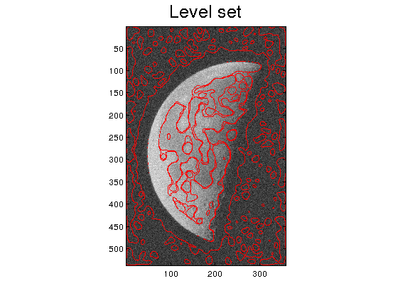
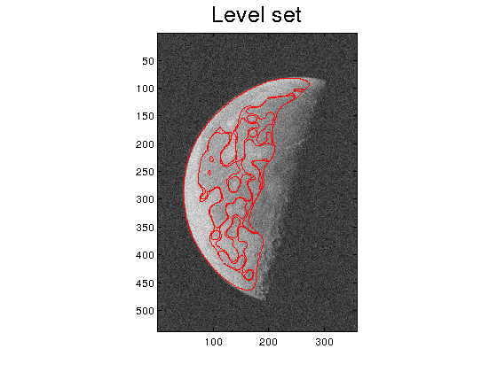
Step 4. Observe that due to the noise, there are spurious borders in the background. For this particular image, they are easy to remove by thresholding the smoothed image:
I2=I2.*(I2>0.5);
and then applying Steps 2 and 3
example2
Exercise 2 We perform a similar analysis but using the zero crossing of the gradient: \[ DI=\sqrt{(DxI)^2+(DyI)^2}\] where \(DxI\) and \(DyI\) are computed through convolution of the image with the kernels \[kx=0.5\left(\begin{array}{ccc} 0 & 0 & 0 \\-1 & 0 & 1 \\0 & 0 & 0 \end{array}\right) \quad\quad\quad ky=0.5\left(\begin{array}{ccc} 0 & -1 & 0 \\0 & 0 & 0 \\0 & 1 & 0 \end{array}\right) \]
Repit Steps 1-4 above introducing the following changes:
- Load the Matlab image coins.png and set noise=0.5.
- Play with the number of iterations in Step 2, and visualize some of them to understand how the smoothing effect works.
- In Step 3, implement the zero-crossing filter for \(DI\). In this case, set threshold=0.01.
- Use the smoothed image thresholding of Step 4
Exercise2