Linear systems
Contents
Introduction
In this lab we tackle the problem of solving linear systems of equations \[ \begin{array}{cll} a_{11}x_{1}+a_{12}x_{2}+\ldots+a_{1n}x_{n} & = & b_{1},\\ a_{21}x_{1}+a_{22}x_{2}+\ldots+a_{2n}x_{n} & = & b_{2},\\ \vdots\\ a_{n1}x_{1}+a_{n2}x_{2}+\ldots+a_{nn}x_{n} & = & b_{n}. \end{array} \] We assume that the matrix \(A=(a_{ij})\) is non-singular, i.e. \(det A\) does not vanish, and therefore, the system has a unique solution.
Direct methods
LU decomposition
We express \(A\) as a matrix multiplication of two matrices: a Lower triangular matrix, \(L\), and an Upper triangular matrix, \(U\), \[ A=LU. \] Consider the system \[ A\mathbf{x}=\mathbf{b}, \] where \(A\) admits the \(LU\) decomposition. Then \[ A\mathbf{x}=\mathbf{b}\Longleftrightarrow LU\mathbf{x}=\mathbf{b} \] Using the Matlab command lu
A=[2 1 1;1 2 -1;-1 1 2];
[L U P]=lu(A)
L =

    1.0000         0         0
    0.5000    1.0000         0
   -0.5000    1.0000    1.0000


U =

    2.0000    1.0000    1.0000
         0    1.5000   -1.5000
         0         0    4.0000


P =

     1     0     0
     0     1     0
     0     0     1
The matrix \(P\) is introduced to store the row reordering, so we have \(PA=LU\). Then, solving \(PAx=Pb\) is equivalent to solving \(Ax=b\), which is done in two steps
- Solve \(L\mathbf{y}=P\mathbf{b}\), by forward substitution, to get \(\mathbf{y}\).
- Solve \(U\mathbf{x}=\mathbf{y}\), by backward substitution, to get \(\mathbf{x}\).
FORWARD SUBSTITUTION
For the system \[ L\mathbf{x}=\mathbf{b}, \] with \(L\) of the form \[ L=\left(\begin{array}{ccccc} l_{11} & 0 & 0 & \ldots & 0\\ l_{21} & l_{22} & 0 & \ldots & 0\\ l_{31} & l_{32} & l_{33} & \ldots & 0\\ \vdots & \vdots & \vdots & \ddots & \vdots\\ l_{n1} & l_{n2} & l_{n3} & \ldots & l_{nn} \end{array}\right) \] the \(i\)-th equation is, for \(i=1,2,\ldots,n\), \[ l_{i1}x_{1}+l_{i2}x_{2}+\cdots+l_{ii}x_{i}=b_{i}. \]
Therefore, for \(i=1,2,\ldots,n\), if \(l_{ii}\) does not vanish, then \[ x_{i}=\frac{b_{i}-l_{i1}x_{1}-\cdots-l_{ii-1}x_{i-1}}{l_{ii}}= \frac{1}{l_{ii}}\left(b_{i}-\sum_{j=1}^{i-1}l_{ij}x_{j}\right). \]
Algorithm
- If \(l_{11}=0\), exit
- Set \(x_{1}=\frac{b_{1}}{l_{11}}\)
- For \(i=2,\ldots,n\)
- -----If \(l_{ii}=0\), exit
- -----Set \[ x_{i}=\frac{1}{l_{ii}}\left(b_{i}-\sum_{j=1}^{i-1}l_{ij}x_{j}\right). \]
Exercise 1. Write a function x=sust_forward(L,b) where \(x\) is the solution of the system \(Lx=b\), for \(L\) lower triangular. Solve the system \[\left(\begin{array}{rrr} 2 & 0 & 0\\ 1 & 2 & 0\\ 1 & 1 & 2 \end{array}\right) \left(\begin{array}{c} x_1\\ x_2\\ x_3 \end{array}\right)= \left(\begin{array}{r} 2\\ -1\\ 0 \end{array}\right) \]
L=[2 0 0;1 2 0;1 1 2];
b=[2 -1 0];
x=sust_forward(L,b')
x =

     1
    -1
     0
BACKWARD SUBSTITUTION
Similarly, for the system \[ U\mathbf{x}=\mathbf{b}' \] with \(U\) of the form \[ U=\left(\begin{array}{ccccc} u_{11} & u_{12} & u_{13} & \ldots & u_{1n}\\ 0 & u_{22} & u_{23} & \ldots & u_{2n}\\ 0 & 0 & u_{33} & \ldots & u_{3n}\\ \vdots & \vdots & \vdots & \ddots & \vdots\\ 0 & 0 & 0 & 0 & u_{nn} \end{array}\right) \] the \(i\)-th equation is, for \(i=1,2,\ldots,n\), \[ u_{ii}x_{i}+u_{ii+1}x_{i+1}+\cdots+u_{in}x_{n}=b_{i} \] Therefore, for \(i=1,2,\ldots,n\), if \(l_{ii}\) does not vanish then \[ x_{i}=\frac{b_{i}-u_{ii+1}x_{i+1}-\cdots-u_{in}x_{n}}{u_{ii}}= \frac{1}{u_{ii}}\left(b_{i}-\sum_{j=i+1}^{n}u_{ij}x_{j}\right), \]
Algorithm
- If \(u_{11}=0\), exit
- Set \(x_{n}=\frac{b_{n}}{u_{nn}}\)
- For \(i=n-1,\ldots,1\)
- ---- If \(u_{ii}=0\), exit
- ---- Set \[ x_{i}=\frac{1}{u_{ii}}\left(b_{i}-\sum_{j=i+1}^{n}u_{ij}x_{j}\right). \]
Exercise 2. Write a function x=sust_backward(L,b) where \(x\) is the solution of the system \(Ux=b\), for \(U\) upper triangular. Solve the system \[\left(\begin{array}{rrr} 2 & 1 & 1\\ 0 & 2 & 1\\ 0 & 0 & 2 \end{array}\right) \left(\begin{array}{c} x_1\\ x_2\\ x_3 \end{array}\right)= \left(\begin{array}{r} 9\\ 4\\ 4 \end{array}\right) \]
L=[2 1 1;0 2 1;0 0 2];
b=[9 4 4];
x=sust_backward(U,b')
x =

    2.1667
    3.6667
    1.0000
Exercise 3. Use the \(LU\) decomposition of \(A\) to solve the system \(Ax=b\), with \[ A=\left(\begin{array}{rrr} 2 & 1 & 1\\ 1 & 2 & 2\\ 1 & 1 & 2 \end{array}\right)\quad\quad b=\left(\begin{array}{c} 2\\ 4\\ 6 \end{array}\right) \]
Exercise3
L =

    1.0000         0         0
    0.5000    1.0000         0
    0.5000    0.3333    1.0000


U =

    2.0000    1.0000    1.0000
         0    1.5000    1.5000
         0         0    1.0000


P =

     1     0     0
     0     1     0
     0     0     1


b1 =

     2
     4
     6


y =

     2
     3
     4


x =

     0
    -2
     4
Iterative methods
Iterative methods are, in general, more efficient than direct methods for solving sparse large systems of linear equations.
We rewrite the problem as \[ A\mathbf{x}=\mathbf{b}\Longleftrightarrow\mathbf{x}=B\mathbf{x}+\mathbf{c} \] where \(B\) is a matrix of order \(n\) and \(c\) is a column vector of dimension \(n\).
Then, if \(\mathbf{x}^{(0)}\) is an initial guess, for \(k=1,2,\ldots\) \[ \mathbf{x}^{(k)}=B\mathbf{x}^{(k-1)}+\mathbf{c} \]
METHOD OF JACOBI
Algorithm
- Choose an initial guess \(\mathbf{x}^{(0)}\)
- For \(k=1,2,\ldots,MaxIter\)
- ----For \(i=1,2,\ldots,n\) compute \[ x_{i}^{(k)}=\frac{1}{a_{ii}}(b_{i}-\sum_{j=1}^{i-1}a_{ij}x_{j}^{(k-1)}-\sum_{j=i+1}^{n}a_{ij}x_{j}^{(k-1)}) \]
- ----If the stopping criterium is satisfied, take \(\mathbf{x}^{(k)}\) as approximated solution
Exercise 4. Write a function x=jacobi(A,b,tol) to solve \(Ax=b\) by Jacobi's method.
Solve \[ \begin{cases} 5x_{1}+x_{2}-x_{3}-x_{4} & =1\\ x_{1}+4x_{2}-x_{3}+x_{4} & =1\\ x_{1}+x_{2}-5x_{3}-x_{4} & =1\\ x_{1}+x_{2}+x_{3}-4x_{4} & =1 \end{cases} \] by Jacobi's method, for a relative tolerance of \(10^{-6}\).
A=[ 5 1 -1 -1; 1 4 -1 1 ; 1 1 -5 -1; 1 1 1 -4];
b=[1;1;1;1];
tol=1e-6;
x=jacobi(A,b,tol)
x =

    0.0937
    0.2500
   -0.0937
   -0.1875
METHOD OF GAUSS-SEIDEL
Algorithm
- Choose an initial guess \(\mathbf{x}^{(0)}\)
- For \(k=1,2,\ldots,MaxIter\)
- ----For \(i=1,2,\ldots,n\) compute \[ x_{i}^{(k)}=\frac{1}{a_{ii}}(b_{i}-\sum_{j=1}^{i-1}a_{ij}x_{j}^{(k)}-\sum_{j=i+1}^{n}a_{ij}x_{j}^{(k-1)}) \]
- ----If the stopping criterium is satisfied, take \(\mathbf{x}^{(k)}\) as approximated solution
Exercise 5. Write a function x=jacobi(A,b,tol) to solve \(Ax=b\) by Gauss-Seidel's method. Solve the system above.
x=gauss_seidel(A,b,tol)
x =

    0.0937
    0.2500
   -0.0938
   -0.1875
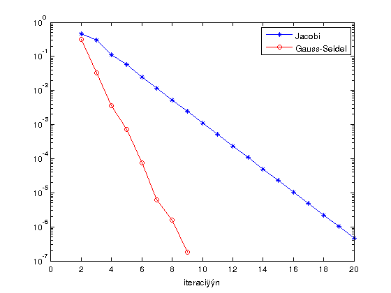
Exercise 6. Modify the above functions using the file names jacobi2 and gauss_seidel2, to get the sequences of approximated solutions and their corresponding relative errors. Use them to:
- Plot the sequence of errors in logarithmic scale (command semilogy) for both methods
Exercise6
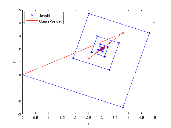
- Solve by Jacobi and Gauss-Seidel the system \[ \begin{cases} 5x+2y & =19\\ 3x-2y & =5 \end{cases} \] with relative tolerance \(10^{-2}\) and plot the sequence of approximated solutions in the plane XY.
Exercise7
The Matlab command \
Example
Solve the system of Exercise 4 using the Matlab command \
A=[ 5 1 -1 -1; 1 4 -1 1 ; 1 1 -5 -1; 1 1 1 -4];
b=[1;1;1;1];
x=A\b
x =

    0.0937
    0.2500
   -0.0938
   -0.1875