Applications of Optimization. Denoising algorithms

Contenidos

Gradient descent for unconstrained problems
A first general example
Image denoising

Gradient descent for unconstrained problems

We consider the problem of finding a minimum $x^*\in\mathbb{R}^N$ of a function $f:\mathbb{R}^N\to\mathbb{R}$, i.e. of solving \[ \min_{x\in\mathbb{R}^N} f(x) \] Note that the minimum is not necessarily unique. In general, there might exist several local minima. However, under the assumption of convexity, the minimum is unique and the algorithms based on descent techniques converge to the global minimizer.

The simplest method is the gradient descent which, for $k=0,1,\ldots$ computes \[ x^{(k+1)}=x^{(k)}- \tau \nabla f(x^{(k)}), \] where $\tau$ is the step size. An initial guess, $x^{(0)}$ is assumed to be given.

A first general example

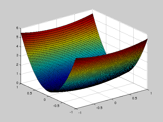
It is clear that the convex function $f(x)=\frac{1}{2}(x_1^2+\eta x_2^2)$ where $\eta>0$ is a fixed number, has a global minimum at the origin $(x_1,x_2)=(0,0)$.

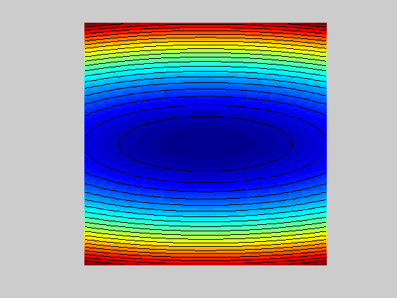
To apply the gradient descent method, we start by fixing $\eta$ and defining $f$. We also produce some graphic representations.

eta=10;
f = @(x1,x2)( x1.^2 + eta*x2.^2 ) /2;
t = linspace(-1,1,101);
[u,v] = meshgrid(t,t);
F=f(u,v);
figure,surf(u,v,F)
figure,hold on;imagesc(t,t,F); contour(t,t,F, 20, 'k');
axis off; axis equal;hold off

We implement the gradient descent. The gradient is computed analitically.

Gradf = @(x)[x(1); eta*x(2)];
tau = 1.8/eta;                  % define the step size
x=[0.5,0.5]';                   % initial guess
X=x;                            % initialize sequence x^k
for k=1:20
     x=x-tau*Gradf(x);
     X=[X x];
end

We show in two graphics the path of the minimizing sequence in the contour plot of function $f$, and how $f(x^{(k)})$ decreases along this path.

figure,hold on;
imagesc(t,t,F); contour(t,t,F, 20, 'k');plot(X(1,:), X(2,:), 'w.-');
axis off; axis equal;title('path of minimiziing sequence')
hold off
f_descent=f(X(1,:),X(2,:));
figure,plot(f_descent),title('descent path of function f')

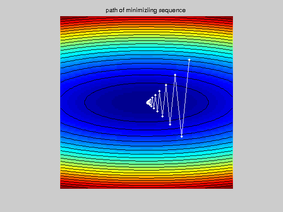
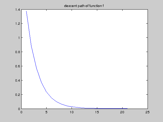
Image denoising

Instead of looking for a minimizing sequence of points $x^{(k)}\in\mathbb{R}^N$ for a function $f:\mathbb{R}^N\to\mathbb{R}$, we look for a minimizing sequence of images $u^{(k)}(x)$, for a functional $J:V\to\mathbb{R}$, where $V$ is the space of images (a space of smooth functions).

We consider functionals $J$ which are the addition of two terms, $J=J_1+J_2$. The first term is the fidelity term which forces the final image to be not too far away from the initial image. The second term is the regularizing term, which performs actually the noise reduction.

A typical choice of the fidelity term is the convex functional \[J_1(u)=\frac{1}{2} \|u-u_0\|^2= \frac{1}{2}\int_{\Omega}|u(x)-u_0(x)|^2dx\] where $\Omega$ denotes the set of pixels and $u_0$ is the initial image.

For the regularizing term, we start with the simplest choice (also convex) \[J_2(u)=\frac{1}{2} \|\nabla u\|^2= \frac{1}{2}\int_{\Omega}|\nabla u(x)|^2dx\]

Then the problem is: find a minimum $u^*\in V$ of $J:V\to\mathbb{R}$, i.e. solving \[ \min_{u\in V} \frac{1}{2}\int_{\Omega}|u(x)-u_0(x)|^2dx+ \lambda\frac{1}{2}\int_{\Omega}|\nabla u(x)|^2dx .\] Here, $\lambda>0$ is a parameter to control the rate fidelity-regularization.

For using the gradient descent method we need to compute the gradient of $J$. The result is \[ \nabla J(u(x))= u(x)-u_0(x) -\lambda\Delta u(x) .\] Then, the gradient descent algorithm gives \[ u^{(k+1)}(x)=u^{(k)}(x)-\tau \big( u^{(k)}(x)-u_0(x) -\lambda\Delta u^{(k)}(x) \big) \]

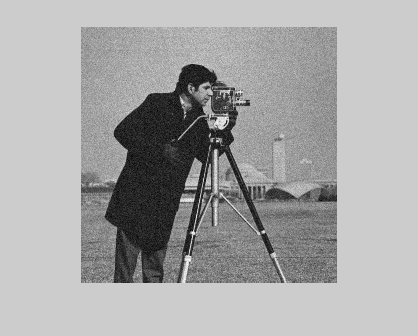
Example. Let us consider the cameraman image

clear all
I=imread('cameraman.tif');

to which we add some noise and transform to double precission for computing. We also normalize the image to take intensity values in $[0,1]$

u0=im2double(I)+0.05*randn(size(I));
u0=(u0-min(min(u0)))/(max(max(u0))-min(min(u0)));

We define the initial step and compute the sequence, renormalizing the imge in each iteration

tau=0.1;
lambda=2;
u=u0;
for k=1:20
    [ux,uy]=gradient(u);
    u=u-tau*(u-u0-lambda*divergence(ux,uy));
    u=(u-min(min(u)))/(max(max(u))-min(min(u)));
end
figure,imshow(u0)
figure,imshow(u)

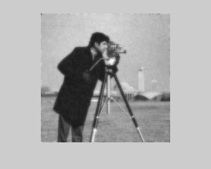
Exercise 8.1 The amount of relative error added to the clean image is about $5\%$. Compute the relative difference between $u_0$ and $u$ for different values of $\tau$, say $\tau=0:0.005:0.1$, and make a plot of it. Visually, which error is better for the denoising result?

Exercise 8.2 Introduce a stopping criterium in terms of the relative difference between two iterations in the above scheme.

Exercise 8.3 In the Total Variation algorithm, we replace $J_2$ given above by \[ J_2(u) = \int_\Omega \|\nabla u(x)\| dx .\] Its gradient is given by \[ \nabla J_2(u) = \frac{\nabla u(x)}{\|\nabla u(x)\|}. \] Since in the regions where $\nabla u(x) =0$ this may be not well defined, we introduce the following approximation \[ \nabla J_{2\epsilon}(u) = \frac{\nabla u(x)}{\sqrt{\epsilon^2+\|\nabla u(x)\|^2}}. \] Use the following parameters in your program: $\lambda=0.1$, $\tau=0.1$, $\epsilon=0.001$. The result is

exercise8_3

You may observe that the blurring effect is less evident and the general denoising has been improved.