Numerical integration
Contents
Quadrature formulas
Numerical integration or quadrature formulas
$$ \int_{a}^{b}f(x)\,dx\approx \omega_{0}\;f(x_{0})+\omega_{1}\;f(x_{1})+\cdots +\omega_{n}\;f(x_{n}) $$where $x_{0},x_{1},...,x_{n}$ (nodes) are $n+1$ different points in the interval $[a,b]$ and $\omega_{0},\omega_{1},\ldots ,\omega_{n}$ (weights) are real numbers.
Interpolatory quadrature formulas
If $P_{n}$ is the polynomial interpolation function for $f$ in the nodes $x_{0},x_{1},...,x_{n} \in \left[ a,b\right]$ and
$$ \int_{a}^{b}f(x)\,dx\approx \int_{a}^{b}P_n(x)\, dx=\omega_{0}\,f(x_{0})+\omega_{1}\,f(x_{1})+\cdots +\omega_{n}\,f(x_{n}) $$this is called an interpolatory quadrature formula.
Simple and composite quadrature formulas
Quadrature formulas are called simple if the approximation takes place in the whole interval $(a,b),$ and composite if, before the application of the formula, we split the interval $(a, b)$ in a given number, $n,$ of subintervals.
Degree of precision
The degree of precision is used for simple quadrature formulas. A quadrature formula has degree of precision $r$ if the rule is exact for
$$ f\left( x\right) =1,\quad f\left( x\right) =x,\quad f\left( x\right) =x^{2},...,\quad f\left( x\right) =x^{r}$$and it is not for $f\left( x\right) =x^{r+1}$
Simple Newton-Cotes formulas
They are interpolatory quadrature formulas where the nodes are equispaced within the interval. There are two types of Newton-Cotes formulas
- Closed formulas. The integration limits $a$ and $b$ are nodes.
- Open formulas. The integration limits $a$ and $b$ are not nodes.
Write the function plotting(f,a,b,nodes) whose input parameters are the lambda function f we will integrate in the interval with boundaries a and b, and the nodes to build the interpolatory formula are in the array nodes that plots
- The area calculated by the integral.
- The nodes.
- The approximate area calculated by the interpolatory formula that uses the nodes.
Check the formula with
- $f(x) = e^x$, $[a,b]=[0,3]$ and
nodes = np.array([1,2,2.5]) - $f(x) = \cos(x) + 1.5$, $[a,b]=[-3,3]$ and
nodes = np.array([-3.,-1,0,1,3])
Hint
- If we want to plot a polygonal line that joins the points $(x_0,y_0),$ $(x_1,y_1)$ and $(x_2,y_2)$ with a dashed red line
plt.plot([x0,x1,x2],[y0,y1,y2],'r--')
%run Exercise1plot


Let us compute first the exact integral
We import the modules numpy y sympy
import numpy as np
import sympy as sym
And the exact value of
$$ \int_1^3 \ln(x) \,dx \qquad (1) $$is
x = sym.Symbol('x', real=True)
f_sym = sym.log(x)
Ie = sym.integrate(f_sym,(x,1,3))
print(Ie)
We also can express it as
Ie = float(Ie)
print(Ie)
Midpoint rule
The Midpoint rule is
$$\int_{a}^{b}f(x)\,dx\approx (b-a)\;f\left( \frac{a+b}{2}\right)$$The formula can be generated substituting the function inside the integral by the zero degree polynomial that passes throught the point of the curve in the center of the $[a,b]$ interval; that is, the horizontal line that passes throught the middle point of the function. Geometrically, we are computing the area of a rectangle.
Write a midpoint(f,a,b) function whose input are the function f and the boundaries of the integration interval a and b, and the output, the approximate value of the integral using the Middle Point rule. Compute the integral
Print the exact value (calculated above) and the approximate value.
%run Exercise1a.py

Trapezoidal rule
The simple Trapezoidal rule is
$$\int_{a}^{b}f(x)\,dx\approx \frac{b-a}{2}\;\left( f\left( a\right) +f\left( b\right) \right)$$The formula can be generated substituting the function inside the integral by the one degree polynomial that passes throught the points of the curve in the boundaries of the $[a,b]$ interval; that is, the line that passes throught two boundary points of the function in the interval. Geometrically, we are computing the area of a trapezoid.
Write a trapez(f,a,b) function whose input are the function f and the boundaries of the integration interval a and b, and the output, the approximate value of the integral using the Trapezoidal rule. Compute the integral
Print the exact value and the approximate value.
%run Exercise1b.py

Simpson's rule
Simpson's rule is
$$\int_{a}^{b}f(x)\,dx\approx \frac{b-a}{6}\;\left( f\left( a\right) +4\;f\left( \frac{a+b}{2}\right) +f\left( b\right) \right)$$The formula can be generated substituting the function inside the integral by the two degree polynomial that passes throught three points of the curve in the boundaries and the middle point of the $[a,b]$ interval; that is, the parabola that passes throught these three pointsin the interval. Geometrically, we are computing the area under the parabola.
Write a simpson(f,a,b) function whose input are the function f and the boundaries of the integration interval a and b, and the output, the approximate value of the integral using the Simpson rule. Compute the integral
Print the exact value and the approximate value.
%run Exercise1c.py

Composite Newton-Cotes formulas
A way to decrease the error is to increase the number of nodes using the composite rules. They are obtained splitting the interval $\left[ a,b\right] $ in $n$ subintervals and using, for each of this subintervals, the simple quadrature rule.
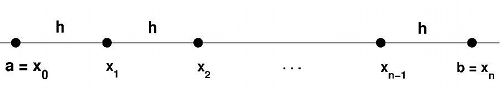
If we divide the interval $\left[ a,b\right] $ into $n$ subintervals of equal length using the nodes $x_{0},x_{1},...,x_{n}$,
the length of a subinterval is
$$h=\frac{b-a}{n}$$the nodes are
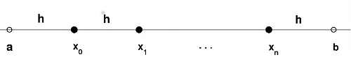
$$x_i=a+i\,h \quad i=0,1,\ldots,n$$and the middle point of a subinterval is
$$\bar x_i =\frac{x_{i-1}+x_i}{2}$$then, the composite formulas can be written:
Composite Midpoint rule
$$ \int_a^b f(x)\, dx \approx h\sum_{i=1}^{n}f(\bar x_i)$$Write a comp_midpoint(f,a,b,n) function whose input are the function f and the boundaries of the integration interval a and b, and n the number of subintervals, and the output, the approximate value of the integral using the composite Middle Point rule. Compute, with n = 5 subintervals the integral
Print the exact value and the approximate value.
%run Exercise1d.py

Composite Trapezoidal rule
$$ \int_a^b f(x)\, dx \approx \frac{h}{2}(f(a)+f(b))+h\sum_{i=1}^{n-1}f(x_i)$$Write a comp_trapz(f,a,b,n) function whose input are the function f and the boundaries of the integration interval a and b and n the number of subintervals, and the output, the approximate value of the integral using the composite Trapezoidal rule. Compute, with n = 4 subintervals the integral
Print the exact value and the approximate value.
%run Exercise1e.py

Composite Simpson's rule
$$ \int_a^b f(x)\, dx \approx \frac{h}{6}\sum_{i=1}^{n}\left(f(x_{i-1})+4f(\bar x_i)+f(x_i)\right)) $$Write a comp_simpson(f,a,b,n) function whose input are the function f and the boundaries of the integration interval a and b and n the number of subintervals, and the output, the approximate value of the integral using the composite Simpson rule. Compute, with n = 4 subintervals the integral
Print the exact value and the approximate value.
%run Exercise1f.py

Gaussian quadrature formulas
In the quadrature formula
$$ \int_{a}^{b}f(x)\,dx\approx \omega_{0}\,f(x_{0})+\omega_{1}\,f(x_{1})+\cdots +\omega_{n}\,f(x_{n}) $$Is is possible to compute the weights $\omega_i$ and the nodes $x_i$ so the precision of the formula is maximum? Yes, but then, the nodes are not equispaced.
If we have $n$ nodes in $[a,b]=[-1,1]$ the weights and the nodes are
These nodes and weights can be obtained with np.polynomial.legendre.leggauss(n). For instance, if $n = 1$:
n = 1
[x, w] = np.polynomial.legendre.leggauss(n)
print('w\n',w)
print('x\n',x)
For instance, the gaussian formula with one node
$$ \int_{-1}^{1}f(x)\,dx\approx 2\;f(0) $$that it is the same as the Middle Point rule. For two nodes
n = 2
[x, w] = np.polynomial.legendre.leggauss(n)
print('w\n',w)
print('x\n',x)
For three nodes
n = 3
[x, w] = np.polynomial.legendre.leggauss(n)
print('w\n',w)
print('x\n',x)
And so on.
This formulas can be generalized for any interval $[a,b]$ changing $x_i$ with $y_i$ following the
$$y_i=\frac{b-a}{2}x_i+\frac{a+b}{2}$$And then, the quadrature formula is
$$ \int_{a}^{b}f(x)\,dx\approx\frac{b-a}{2}\left( \omega_{0}\;f(y_{0})+\omega_{1}\;f(y_{1})+\cdots +\omega_{n}\;f(y_{n})\right) $$Write a gauss(f,a,b,n) function whose input are the function f and the boundaries of the integration interval a and b and n the number of interpolation points, and the output, the approximate value of the integral using the gaussian formula. Compute, with n = 1, n = 2 and n = 3 nodes the integral
Print the exact value and the approximate value.
%run Exercise2.py


Degree of precision of a quadrature formula
The degree of precision is used for simple quadrature formulas. A quadrature formula has degree of precision $r$ if the rule is exact for
$$ f\left( x\right) =1,\quad f\left( x\right) =x,\quad f\left( x\right) =x^{2},...,\quad f\left( x\right) =x^{r}$$and it is not for $f\left( x\right) =x^{r+1}$
Write a function newton_cotes(f,a,b,n) that returns the value of the approximate integral of $f$ in the interval $[a,b]$ with the function midpoint if n = 1, trapez if n = 2 and simpson if n = 3 where n is the number of nodes used in the formula.
Write a function degree_of_precision(formula,n) function whose input is the function newton_cotes or gauss, and n is the number of nodes used in the formula, that studies the degree of precision of these quadrature formulas, computing their error for the integrals
and when the error is less than zero, it stops. Print the erros for each polynomial and the degree of precision of the formula.
Notes:
- Due to the rounding errors, consider that the actual error is zero when the obtained error is less than $10^{-10}$.
%run Exercise3.py
More exercises
Numerical integration with python commands
The module scipy.integrate contains different integrating functions. For instance, the function quad
import scipy.integrate as inte

f = lambda x : np.log(x)
a = 1.; b = 3;

I = inte.quad(f,a,b)

print ('The approximate value is ', I[0])
print ('The exact value is       ', I_exacta)
Montecarlo integration
We can compute an integral using random numbers.
Let us begin with a positive function in the integration interval $[a,b]$. The value of the integral is then the area between the curve and the OX axis. We compute this area:
- We obtain "n" random points within the rectangle $[a,b]\times[0,\max (f)].$
- We count the number of points between the curve and the OX axis.
- The ratio of this number to the total random points multiplied by the rectangle area is the approximate area.
Write a function montecarlo(f,a,b,n) with input arguments f, the function to integer, a and b, the integration interval boundaries and n, the number of random points and output argument, the approximate value of the integral
Print the exact and approximate value of the integral.
Hint
We can obtain n random points uniformly distributed in $[a,b]$ with np.random.rand(n) * (b-a) + a.
%run Exercise4.py

%run Exercise5.py
