k-means algorithm applied to image classification and processing
Classification
Machine Learning applies automatic data-driven learning methods to obtain accurate predictions from observations with previous data.
Data automated classification is one of the aims of machine learning. We can consider three types of classification algorithms:
Supervised classification: We have a dataset (i.e., handwritten digit images) that we will call training data where each datum is associated with a label (that tell us which digit, 0, 1,..,9, corresponds to that image). In the training stage, we build a model with this dataset (training dataset) using the labels, that helps us to assess the correct or incorrect classification of an image while building the model. Once we have the model, we can use it to classify new data. At this stage we do not need the labels, unless we want to assess the accuracy of the classification.
Unsupervised classification: The dataset comes without labels (or we will not use them) and the data is classified using their inner structure (properties, characteristics).
Semi-supervised classification: we can apply it when some data comes with labels, but not all of them. This is typical when our data consist of images: we have access to many images but they are mostly untagged. These algorithms can be considered a variant of the supervised classification with a strategy to overcome the lack of labels for part of the data.
In this lab we will see some application examples of the unsupervised classification algorithm k-means for image classification and processing.
k-means algorithm
K-means is an unsupervised classification algorithm, also called clusterization, that groups objects into k groups based on their characteristics. The grouping is done minimizing the sum of the distances between each object and the group or cluster centroid. The distance usually used is the quadratic or euclidean distance.
The algorithm has three steps:
- Initialization: once the number of groups, k has been chosen, k centroids are established in the data space, for instance, choosing them randomly.
- Assignment of objects to the centroids: each object of the data is assigned to its nearest centroid.
- Centroids update: The position of the centroid of each group is updated taking as the new centroid the average position of the objects belonging to said group.
Repeat steps 2 and 3 until the centroids do not move, or move below a threshold distance in each step.

The k-means algorithm solves an optimization problem and the function to be optimized (minimized) is the sum of the quadratic distances from each object to its cluster centroid.
The objects are represented with $d$ dimension vectors $\left(\mathbf{x}_{1},\mathbf{x}_{2},\ldots,\mathbf{x}_{n}\right)$ and the algorithm k-means builds $k$ groups where the sum of the distances of the objects to its centroid is minimized within each group $\mathbf{S}=\left\{ S_{1},S_{2},\ldots,S_{k}\right\}$. The problem can be formulated:
where $\mathbf{S}$ is the dataset whose elements are the objects $\mathbf{x}_{j}$ represented by vectors, where each of its elements represents a characteristic or attribute. We will have $k$ groups or clusters with their corresponding centroid $\boldsymbol{\mu_{i}}$.
In each centroid update, from the mathematical point of view, we impose the extreme (minimum, in this case) necessary condition to the function $E\left(\boldsymbol{\mu_{i}}\right)$ that, for this quadratic function $(1)$ is
and the solution is to take each group element average as a new centroid. We have used the gradient descent method.
The main advantages of the k-means method are that it is simple and fast. But it is necessary to decide the value of $k$ and the final result depends on the initialization of the centroids. Also, it does not necessarily converge to the global minimum but to a local minimum.
Write a script that uses the k-means method to classify two dimensional data. Classify the data generated below in three groups.

We generate 2D random data for three clusters with the function
def generate_data():
np.random.seed(7)
x1 = np.random.standard_normal((100,2))*0.6+np.ones((100,2))
x2 = np.random.standard_normal((100,2))*0.5-np.ones((100,2))
x3 = np.random.standard_normal((100,2))*0.4-2*np.ones((100,2))+5
X = np.concatenate((x1,x2,x3),axis=0)
return X
We generate the $k=3$ initial centroids in $[0,1]\times [0,1]$ with the function
def generate_centroids(X,k):
cx = np.random.rand(k)
cy = np.random.rand(k)
centroids = np.zeros((k,2))
centroids[:,0] = cx
centroids[:,1] = cy
return centroids
If we want to scale a value $x$ from $[0,1]$ to $[a,b]$
$$x_s = a + (b-a)\,x$$(a) Modify the previous function in such a way that the cx values are between the maximum and minimum value of the first coordinate in X. And the cy values are between the maximum and minimum value of the first coordinate in X.
Note np.min(v) and np.max(v) give the minimum and maximum value of an unidimensional vector v.
(b) Create a function assign_centroid(x,centroids) that given a point of the data (a row of X) returns in l the row of the nearest centroid. Use the euclidean distance.
(c) Create a function reallocate_centroids(X,labels,centroids) that recalculates the centroids as average values of the X point whose label corresponds with the row of the centroid.
(d) Create a funcion kmeans(k) that, calling the adequate functions:
- Generates the data.
- Generates the centroids.
- Initializes the one-dimensional numpy array
labelswith the length the number of points inXwith 9. - Plots the data with the initial centroids.
- Assigns centroids to the points and plot the clusters.
- Reallocates the centroids and plot them with the clusters.
Repeat steps 5 and 6 eight times
Plot the data and the centroids using the following function.
def plot_data(X,labels,centroids,s):
plt.figure()
plt.plot(X[labels==9,0],X[labels==9,1],'k.')
plt.plot(X[labels==0,0],X[labels==0,1],'r.', label='cluster 1')
plt.plot(X[labels==1,0],X[labels==1,1],'b.', label='cluster 2')
plt.plot(X[labels==2,0],X[labels==2,1],'g.', label='cluster 3')
plt.plot(centroids[:,0],centroids[:,1],'mo',markersize=8, label='centroids')
plt.legend()
plt.title(s)
plt.show()
%run Exercise1.py


import numpy as np
import matplotlib.pyplot as plt
We will use KMeans from sklearn library in the other exercises.
from sklearn.cluster import KMeans
We group the points with k-means and $k=3$
n = 3
X = generate_data()
k_means = KMeans(n_clusters=n)
model = k_means.fit(X)
The result is three centroids around which the points are grouped and each point label that indicate which cluster this point belongs to.
centroids = k_means.cluster_centers_
labels= k_means.labels_
Now we draw the points and the centroids, using a different color for the points of each cluster.
plt.figure()
plt.plot(X[labels==0,0],X[labels==0,1],'r.', label='cluster 1')
plt.plot(X[labels==1,0],X[labels==1,1],'b.', label='cluster 2')
plt.plot(X[labels==2,0],X[labels==2,1],'g.', label='cluster 3')
plt.plot(centroids[:,0],centroids[:,1],'mo',markersize=8, label='centroids')
plt.legend(loc='best')
plt.show()

Digit image classification with k-means
Let us classify digits of the database contained in sklearn library of python using the k-means algorithm.
We import the usual libraries
import numpy as np
import matplotlib.pyplot as plt
and the library that contains the function k-means
from sklearn.cluster import KMeans
We import the library that contains our dataset
from sklearn.datasets import load_digits
We load the digit images
digits = load_digits()
data = digits.data
print(data.shape)
Pixels from the square image of $8\times 8$ pixels have been reshped in a row of $ 64 $ elements. Therefore, each row is an object or data. The characteristics or properties of each object are the gray intensities of each pixel. That is, we have, for each image, $64$ properties.
To improve the visualization, we invert the colors
data = 255-data
We fix the seed to obtain the initial centroids, so the results obtained here are repeatable.
np.random.seed(1)
Since we have 10 different digits (from 0 to 9) we choose to group the images in $10$ clusters
n = 10
We classify the data with k-means
kmeans = KMeans(n_clusters=n,init='random')
kmeans.fit(data)
Z = kmeans.predict(data)
We plot the resulting clusters
for i in range(0,n):
row = np.where(Z==i)[0] # row in Z for elements of cluster i
num = row.shape[0] # number of elements for each cluster
r = int(np.floor(num/10.)) # number of rows in the figure of the cluster
print("cluster "+str(i))
print(str(num)+" elements")
plt.figure(figsize=(10,10))
for k in range(0, num):
plt.subplot(r+1, 10, k+1)
image = data[row[k], ]
image = image.reshape(8, 8)
plt.imshow(image, cmap='gray')
plt.axis('off')
plt.show()


Image quantification with k-means
Quantification is a lossy compression technique that consists of grouping a whole range of values into a single one. If we quantify the color of an image, we reduce the number of colors necessary to represent it and the file size decreases. This is important, for example, to represent an image on devices that only support a limited number of colors.
We import the open vision library OpenCV
import numpy as np
import matplotlib.pyplot as plt
from sklearn.cluster import KMeans
import cv2 as cv
We load the image
I = cv.imread('shop.jpg')
It is a BGR image. We swap channels R and B to have an RGB image
I = cv.cvtColor(I, cv.COLOR_BGR2RGB)
We transform it into a numpy array
a = np.asarray(I,dtype=np.float32)/255
plt.figure(figsize=(12,12))
plt.imshow(a)
plt.axis('off')
plt.show()

In this case our objects are the pixels and their properties are the intensities of red, green and blue associated with each one. Therefore we have as many data or objects as pixels and three features or properties for each pixel. We will have as many different colors as different RGB triple. We count the number of different colors.
First, we get the shape of a. As it is a three dimensional matrix we will have three numbers: the number of pixels in a column, that is the width, same with rows, height, and number of channels.
The number of pixels in the image is w*h
h, w, c = a.shape
print('w =', w)
print('h =', h)
print('c =', c)
num_pixels = w*h
print ('Number of pixels = ', num_pixels)
We create an array with as many rows as pixels and for each row/pixel, 3 columns, one for each color intensity (red, green and blue). We rearrange the matrix this way.
a1 = a.reshape(w*h, c)
print('a shape ', a.shape)
print('a1 shape ', a1.shape)
Now we count the number of unique colors
colors = np.unique(a1, axis=0, return_counts=True)
print(colors)
num_colors = colors[0].shape[0]
print ('\nNumber of colors = ', num_colors)
To apply k-means, we need an array with as many rows as pixels and for each row/pixel, 3 columns, one for each color intensity (red, green and blue). We rearrange the matrix this way. Thus, we will be using a1 that has the adequate shape.
We will group the 172388 colors into 60 groups or new colors, which will correspond to the centroids obtained with the k-means
n = 60
k_means = KMeans(n_clusters=n)
model = k_means.fit(a1)
The final centroids are the new colors and each pixes has been assigned a label the indicates the cluster it belongs.
centroids = k_means.cluster_centers_
labels = k_means.labels_
We reconstruct the matrix of the image from the labels and the colors (intensities of red, green and blue) of thecentroids.
print('centroids shape ', centroids.shape)
print('labels shape ', labels.shape)
a2k = centroids[labels]
print('a2k shape ', a2k.shape)
a3k = a2k.reshape(h, w, c)
print('a3k shape ', a3k.shape)
We view the new image with only 60 colors
plt.figure(figsize=(12,12))
plt.imshow(a3k)
plt.axis('off')
plt.show()

a4k = np.floor(a3k*255)
a5k = a4k.astype(np.uint8)
It is a RGB image. We swap channels R and B to have an BGR image
red = np.copy(a5k[:,:,0])
blue = np.copy(a5k[:,:,2])
a5k[:,:,0] = blue
a5k[:,:,2] = red
We save the image in jpg format
Ik = cv.imwrite("shop2.jpg",a5k)
The number of pixels is the same as in the initial picture but the number of colors in this image is equal to the number of centroids.
colorsk = np.unique(a2k, axis=0, return_counts=True)
num_colorsk = colorsk[0].shape[0]
num_pixelsk = a2k.shape[0]
print('Number of pixels = ',num_pixelsk )
print ('Number of colors = ', num_colorsk)
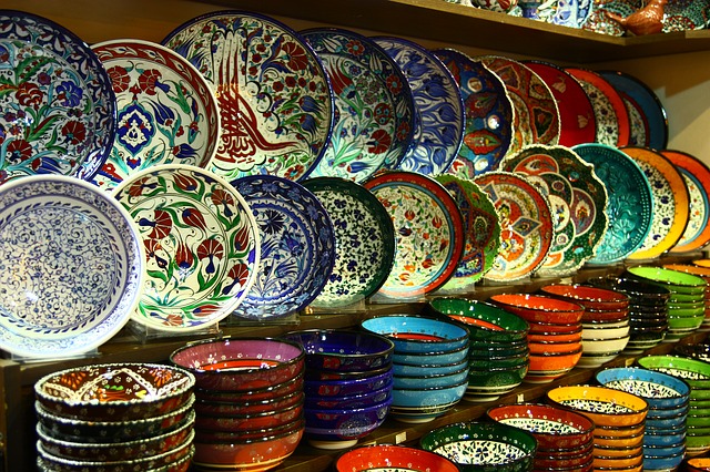
Count the number of colors in the following image, holi.jpg. Create an image where the number of colors has been reduced to 10 using k-means.
Create an $1000\times 1000$ image with the colors of this latter image. Each color will appear as a horizontal band of 100 pixels of width.
Sort the colors by euclidean distance (the distance of a color with the next is the smallest) and plot the set of colors again. Store the image as colors.jpg.
%run Exercise2.py


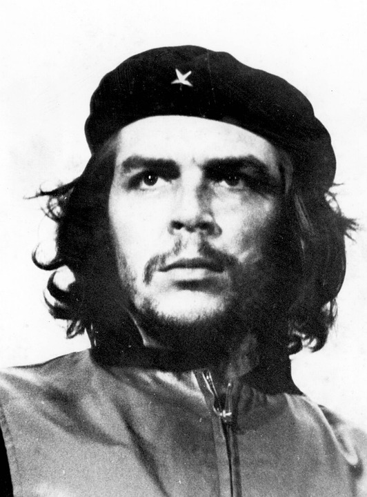
Obtain the third image from the first one (che-guevara.jpg) shown below.
%run Exercise3.py


Image segmentation with k-means
Segmentation divides an image into regions with coherent internal properties. You can segment an image using color.
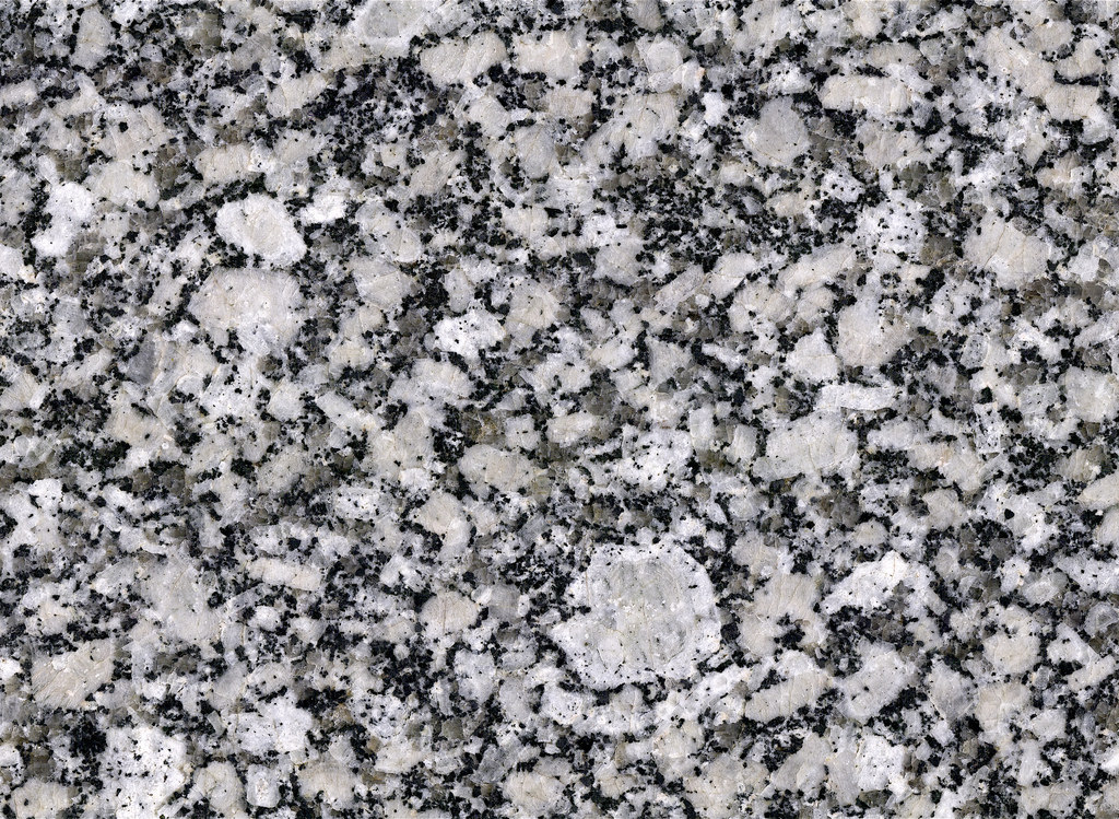
The process is similar to image quantization. The difference is the aim of the pixel grouping: in segmentation, we group the pixels to separate the significant elements of an image and thus, be able to extract certain quantitative information. For example, compute the size of a tumor from medical images, the percentage of mica in a granitic rock, the area of a lake from an aerial photo.
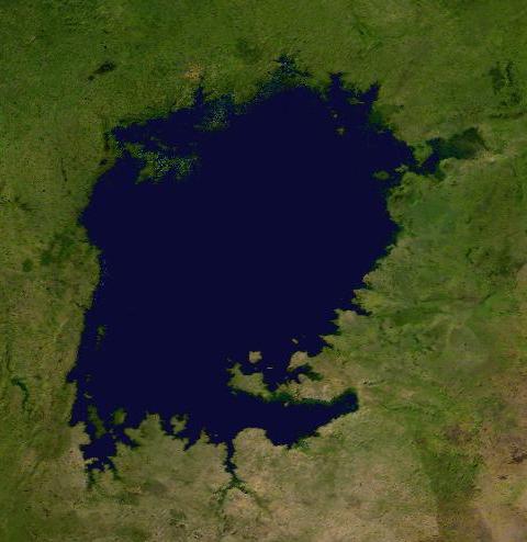
Let us start with this last example. If we have the following image of Lake Victoria taken from a satellite and it covers an area of approximately 200000 km$^2$, we can compute, from the percentage of the area of the image, the area of the lake.
I = cv.imread("VictoriaLake.jpg")
I1 = cv.cvtColor(I, cv.COLOR_BGR2RGB)
plt.figure(figsize=(8,8))
plt.imshow(I1)
plt.axis('off')
plt.show()

To simplify the problem, we convert the color image to black and white
I2 = cv.cvtColor(I, cv.COLOR_BGR2GRAY)
a = np.asarray(I2,dtype=np.float32)
plt.figure(figsize=(8,8))
plt.imshow(a,cmap='gray')
plt.axis('off')
plt.show()

We reshape the matrix to apply k-means. Now it has as many rows as pixels but only one column, the gray intensity.
x , y = a.shape
print('a shape ', a.shape)
a1 = a.reshape(x*y,1)
print('a1 shape ', a1.shape)
We group the pixels into three clusters with k-means
k_means = KMeans(n_clusters=3)
model = k_means.fit(a1)
We extract the centroids and labels for each pixel
centroids = k_means.cluster_centers_
labels = k_means.labels_
We build the image using only the three intensities of the centroids
a2 = centroids[labels]
print('a2 shape ', a2.shape)
a3 = a2.reshape(x, y)
print('a3 shape ', a3.shape)
The rebuilt image
plt.figure(figsize=(8,8))
plt.imshow(a3,cmap='gray')
plt.axis('off')
plt.show()

a4 = (a3 - np.min(a3))/(np.max(a3)-np.min(a3))*255
a5 = a4.astype(np.uint8)
We count the number of pixels of black color (the ones with the lowest gray intensity)
colors = np.unique(a5, return_counts=True)
print(colors)
We have:
print(colors[1][0], 'pixels for intensity',colors[0][0],', that is, black.')
print(colors[1][1], 'pixels for intensity',colors[0][1],', that is, grey.')
print(colors[1][2], 'pixels for intensity',colors[0][2],', that is, white.')
We calculate the percentage of black pixels in the image with respect to the total number of pixels and we have the percentage of the area of the lake with respect to the total area represented by the photo
print ('Area = ', float(200000)*float(colors[1][0])/float(w*h), 'km2')
Calculate the percentage of mica (it is the darkest colored mineral) in the granite rock whose section shows the photo. Execute 10 times the k-means function and keep the iteration that gives the least error with error = k_means.inertia_.
%run Exercise4.py


